Ana içeriğe atla

Excel'de bir önceki veya sonraki belirli bir güne tarih nasıl yuvarlanır?

doc-round-to-önceki-pazar-1
Bazen, gösterilen sol ekran görüntüsü gibi bir tarihe göre Pazar gibi bir önceki veya sonraki belirli hafta içi gününü almanız gerekebilir. İşte bu öğretici, bu işi Excel'de kolayca halletmek için iki formül sağlar.
Sonraki belirli bir hafta içi gününe yuvarlak tarih
Önceki belirli bir hafta içi gününe yuvarlak tarih

ok mavi sağ balon Bir sonraki belirli hafta gününe yuvarlak tarih

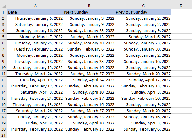
Örneğin, A sütunundaki tarihlerin bir sonraki Pazar gününü almak için burada

1. Sonraki Pazar tarihini yerleştirmek istediğiniz hücreyi seçin, ardından aşağıdaki formülü yapıştırın veya girin:

=IF(MOD(A2-1,7)>7,A2+7-MOD(A2-1,7)+7,A2+7-MOD(A2-1,7))

2. Ardından Keşfet 5 basamaklı bir sayı olarak görüntülenen sonraki ilk Pazar gününü almak için tuşuna basın, ardından tüm sonuçları almak için otomatik doldurmayı aşağı sürükleyin.

doc-round-to-önceki-pazar-1

3. Ardından formül hücrelerini seçili tutun, tuşuna basın. Ctrl + 1 görüntüleme tuşları biçim Hücreler iletişim kutusu, ardından altında Numara sekmesini seçin Tarih ve ihtiyacınız olan şekilde sağ listeden bir tarih türü seçin. Tıklamak OK.

doc-round-to-önceki-pazar-1

Artık formül sonuçları tarih formatında gösterildi.

doc-round-to-önceki-pazar-1

Bir sonraki hafta içi gün almak için lütfen aşağıdaki formülleri kullanın:

çalışma günü formül
Pazar =IF(MOD(A2-1,7)>7,A2+7-MOD(A2-1,7)+7,A2+7-MOD(A2-1,7))
Cumartesi =IF(MOD(A2-1,7)>6,A2+6-MOD(A2-1,7)+7,A2+6-MOD(A2-1,7))
Cuma =IF(MOD(A2-1,7)>5,A2+5-MOD(A2-1,7)+7,A2+5-MOD(A2-1,7))
Perşembe =IF(MOD(A2-1,7)>4,A2+4-MOD(A2-1,7)+7,A2+4-MOD(A2-1,7))
Çarşamba =IF(MOD(A1-1,7)>3,A1+3-MOD(A1-1,7)+7,A1+3-MOD(A1-1,7))
;Salı =IF(MOD(A1-1,7)>2,A1+2-MOD(A1-1,7)+7,A1+2-MOD(A1-1,7))
Pazartesi =IF(MOD(A1-1,7)>1,A1+1-MOD(A1-1,7)+7,A1+1-MOD(A1-1,7))

ok mavi sağ balon Bir önceki belirli hafta gününe yuvarlak tarih

Örneğin, burada A sütunundaki tarihlerin önceki Pazar gününü almak için

1. Sonraki Pazar tarihini yerleştirmek istediğiniz hücreyi seçin, ardından aşağıdaki formülü yapıştırın veya girin:

=A2-HAFTAGÜN(A2,2)

2. Ardından Keşfet sonraki Pazar gününü almak için tuşuna basın, ardından tüm sonuçları almak için otomatik doldurmayı aşağı sürükleyin.

doc-round-to-önceki-pazar-1

Tarih biçimini değiştirmek istiyorsanız, formül hücrelerini seçili tutun, Ctrl + 1 görüntüleme tuşları biçim Hücreler iletişim kutusu, ardından altında Numara sekmesini seçin Tarih ve ihtiyacınız olan şekilde sağ listeden bir tarih türü seçin. Tıklamak OK.

doc-round-to-önceki-pazar-1

Artık formül sonuçları tarih formatında gösterildi.

doc-round-to-önceki-pazar-1

Diğer hafta içi günleri almak için lütfen aşağıdaki formülleri kullanın:

çalışma günü formül
Pazar =A2-HAFTAGÜN(A2,2)
Cumartesi =IF(WEEKDAY(A2,2)>6,A2-WEEKDAY(A2,1),A2-WEEKDAY(A2,2)-1)
Cuma =IF(WEEKDAY(A2,2)>5,A2-WEEKDAY(A2,2)+5,A2-WEEKDAY(A2,2)-2)
Perşembe =IF(WEEKDAY(A2,2)>4,A2-WEEKDAY(A2,2)+4,A2-WEEKDAY(A2,2)-3)
Çarşamba =IF(WEEKDAY(A2,2)>3,A2-WEEKDAY(A2,2)+3,A2-WEEKDAY(A2,2)-4)
;Salı =IF(WEEKDAY(A2,2)>2,A2-WEEKDAY(A2,2)+2,A2-WEEKDAY(A2,2)-5)
Pazartesi =IF(WEEKDAY(A2,2)>1,A2-WEEKDAY(A2,2)+1,A2-WEEKDAY(A2,2)-6)

Güçlü Tarih ve Saat Yardımcısı

The Tarih ve Saat Yardımcısı özelliği Kutools for Excel, tarih saatini kolayca ekleme/çıkarma, iki tarih arasındaki farkı hesaplama ve doğum gününe göre yaşı hesaplamayı destekler.  Ücretsiz deneme için tıklayın!
doc-round-to-önceki-pazar-1
 
Kutools for Excel: 200'den fazla kullanışlı Excel eklentisi ile, hiçbir sınırlama olmaksızın denemek için ücretsiz.

En İyi Ofis Üretkenlik Araçları

🤖 Kutools AI Yardımcısı: Aşağıdakilere dayalı olarak veri analizinde devrim yaratın: Akıllı Yürütme   |  Kodunu oluşturun  |  Özel Formüller Oluşturun  |  Verileri Analiz Edin ve Grafikler Oluşturun  |  Kutools İşlevlerini Çağır...
Popüler Özellikler: Yinelenenleri Bul, Vurgula veya Tanımla   |  Boş Satırları Sil   |  Veri Kaybı Olmadan Sütunları veya Hücreleri Birleştirin   |   Formülsüz Tur ...
Süper Arama: Çoklu Ölçütlü VLookup    Çoklu Değer VLookup  |   Birden Çok Sayfada VLookup   |   Bulanık Arama ....
Gelişmiş Açılır Liste: Hızla Açılır Liste Oluşturun   |  Bağımlı Açılır Liste   |  Çoklu Seçim Açılır Liste ....
Sütun Yöneticisi: Belirli Sayıda Sütun Ekleme  |  Sütunları Taşı  |  Gizli Sütunların Görünürlük Durumunu Değiştir  |  Aralıkları ve Sütunları Karşılaştırın ...
Öne Çıkan Özellikler: Izgara Odağı   |  Tasarım görünümü   |   Büyük Formül Çubuğu    Çalışma Kitabı ve Sayfa Yöneticisi   |  Kaynak Kütüphanesi (Otomatik metin)   |  Tarih Seçici   |  Çalışma Sayfalarını Birleştirin   |  Hücreleri Şifrele/Şifresini Çöz    E-postaları Listeye Göre Gönder   |  Süper Filtre   |   Özel Filtre (kalın/italik/üstü çizili filtre...) ...
En İyi 15 Araç Seti12 Metin Tools (Metin ekle, Karakterleri Kaldır, ...)   |   50+ Grafik Türleri (Gantt şeması, ...)   |   40+ Pratik Formüller (Yaşı doğum gününe göre hesapla, ...)   |   19 sokma Tools (QR Kodunu Girin, Yoldan Resim Ekle, ...)   |   12 Dönüştürme Tools (Sayılardan Kelimelere, Para Birimi Dönüştürme, ...)   |   7 Birleştir ve Böl Tools (Gelişmiş Kombine Satırları, Bölünmüş hücreler, ...)   |   ... ve dahası

Kutools for Excel ile Excel Becerilerinizi Güçlendirin ve Daha Önce Hiç Olmadığı Gibi Verimliliği Deneyimleyin. Kutools for Excel, Üretkenliği Artırmak ve Zamandan Tasarruf Etmek için 300'den Fazla Gelişmiş Özellik Sunar.  En Çok İhtiyacınız Olan Özelliği Almak İçin Buraya Tıklayın...

Açıklama


Office Tab, Office'e Sekmeli Arayüz Getirir ve İşinizi Çok Daha Kolay Hale Getirir

  • Word, Excel, PowerPoint'te sekmeli düzenlemeyi ve okumayı etkinleştirin, Publisher, Access, Visio ve Project.
  • Yeni pencereler yerine aynı pencerenin yeni sekmelerinde birden çok belge açın ve oluşturun.
  • Üretkenliğinizi% 50 artırır ve her gün sizin için yüzlerce fare tıklamasını azaltır!
Comments (16)
No ratings yet. Be the first to rate!
This comment was minimized by the moderator on the site
I have tested this but partially incorrect result was out. Why ?
I wanted to get next Friday.

=IF(A2="","",A2+5-Mod(A2-1,7))

I have entered 11/19/2022
The result was past day 11/18/2022
This comment was minimized by the moderator on the site
Thanks for your reminder, the original formula is not enough rigorous indeed. I have updated the formulas and rewrited the tutorial, hope the new formulas can help you.
This comment was minimized by the moderator on the site
Im trying to work out how to use a date, less an amount of days but ensure when subtracting the days it lands on a weekday not a weekend.
Any formulas??
This comment was minimized by the moderator on the site
Hi Everyone,
I use the formula below to round to the next Thursday where A1 is the cell with your original date and 14 is for Thursday. You can use other numbers for other days if required. 11=Monday, 12=Tuesday, 13=Wednesday, etc...

Also, you can use a 1 instead of an 8 to get the Thursday before your original date in A1. If your original date is already a Thursday the formula will produce the same date as in A1.

I hope this helps!

=A1+(0-WEEKDAY(A1,14)+8)
This comment was minimized by the moderator on the site
Thank you! This worked :)
This comment was minimized by the moderator on the site
I put this into google sheets and to make the dates become next thursday but I have not been able to get it to work especially for the dates right after thursdays. =IF(L2="","",L2+4-MOD(L2-1,4)) is the function i used to make it thursday but not all dates were thursday.
This comment was minimized by the moderator on the site
to clarify, all dates become thursday, but friday and saturday will not convert to the next weeks thursday instead they will go back a day or two to the previous thursday instead going to next weeks thursday, is there any way to fix this in the function =IF(L4="","",L4+4-MOD(L4-1,7))
This comment was minimized by the moderator on the site
Hi Kisho,

I use the formula below to round to the next Thursday where A1 is the cell with your original date and 14 is for Thursday. You can use other numbers for other days if required. 11=Monday, 12=Tuesday, 13=Wednesday, etc...

Also, you can use a 1 instead of an 8 to get the Thursday before your original date in A1. If your original date is already a Thursday the formula will produce the same date as in A1.

I hope this helps!

=A1+(0-WEEKDAY(A1,14)+8)
This comment was minimized by the moderator on the site
Hi Kisho,
I use the formula below to round to the next Thursday where A1 is the cell with your original date and 14 is for Thursday. You can use other numbers for other days if required. 11=Monday, 12=Tuesday, 13=Wednesday, etc...
Also, you can use a 1 instead of an 8 to get the Thursday before your original date in A1. If your original date is already a Thursday the formula will produce the same date as in A1.
I hope this helps!
=A1+(0-WEEKDAY(A1,14)+8)
This comment was minimized by the moderator on the site
I put this into google sheets and to make the dates become next thursday but I have not been able to get it to work especially for the dates right after thursdays. =IF(L2="","",L2+4-MOD(L2-1,4)) is the function i used to make it thursday but not all dates were thursday.
This comment was minimized by the moderator on the site
Si quiero la fecha del próximo viernes cómo debo modificar las variables? Gracias
This comment was minimized by the moderator on the site
Sorry, I cannot understand, could you speak in English?
This comment was minimized by the moderator on the site
hi guys,

I used the formula below, I hope it works for you.
IF(WEEKDAY(H2,16)<>7,(7-WEEKDAY(H2,16))+H2,H2) where H2 is the date that you want to round up to the next day of the week (in my case for Friday) and the 16 is the format to start the date with Saturday as #1 and Friday as #7.
This comment was minimized by the moderator on the site
Your round to previous Sunday is flawed. Even shows as much on your sheet.
This comment was minimized by the moderator on the site
So, what would be the correct formula to first check to see if a cell has a date, else leave it blank and make the date the fall on a Friday before if the date falls on a Saturday or Sunday?
This comment was minimized by the moderator on the site
I found a workaround for to the previous Friday. You can change the switch "results" as needed to round to different days.=H3-SWITCH(TEXT(H3, "DDD"), "Mon", 3, "Tue", 4, "Wed", 5, "Thu", 6, "Fri", 0, "Sat", 1, "Sun", 2)
=[date]-SWITCH(TEXT([date], "DDD"), "Mon", 3, "Tue", 4, "Wed", 5, "Thu", 6, "Fri", 0, "Sat", 1, "Sun", 2)
There are no comments posted here yet
Please leave your comments in English
Posting as Guest
×
Rate this post:
0   Characters
Suggested Locations