Ana içeriğe atla

Excel'de başka bir sütunda aynı değer varsa, hücreleri nasıl birleştirebilirim?

Aşağıdaki ekran görüntüsünde gösterildiği gibi, ikinci sütundaki hücreleri birinci sütundaki aynı değerlere göre birleştirmek istiyorsanız kullanabileceğiniz birkaç yöntem vardır. Bu yazıda, bu görevi gerçekleştirmenin üç yolunu tanıtacağız.

aynıysa birleştir


Formüller ve filtre ile aynı değerde hücreleri birleştirin

Aşağıdaki formüller, bir sütundaki karşılık gelen hücrelerin içeriğini başka bir sütundaki aynı değere göre birleştirmeye yardımcı olur.

1. İkinci sütunun yanında boş bir hücre seçin (burada C2 hücresini seçiyoruz), formülü girin = EĞER (A2 <> A1, B2, C1 & "," & B2) formül çubuğuna girin ve ardından Keşfet tuşuna basın.

2. Ardından C2 hücresini seçin ve Dolgu Tutamaçını birleştirmeniz gereken hücrelere sürükleyin.

3. Formülü girin = EĞER (A2 <> A3, BİRLEŞTİR (A2, "," "", C2, "" ""), "") D2 hücresine girin ve Dolgu Tutamaçını kalan hücrelere sürükleyin.

4. D1 hücresini seçin ve tıklayın Veri > filtre. Ekran görüntüsüne bakın:

5. D1 hücresindeki açılır oku tıklayın, (Boşluklar) ve ardından OK düğmesine basın.

İlk sütun değerleri aynıysa hücrelerin birleştirildiğini görebilirsiniz.

not: Yukarıdaki formülleri başarılı bir şekilde kullanmak için, A sütunundaki aynı değerler sürekli olmalıdır.


Kutools for Excel ile aynı değerde hücreleri kolayca birleştirin (birkaç tıklama)

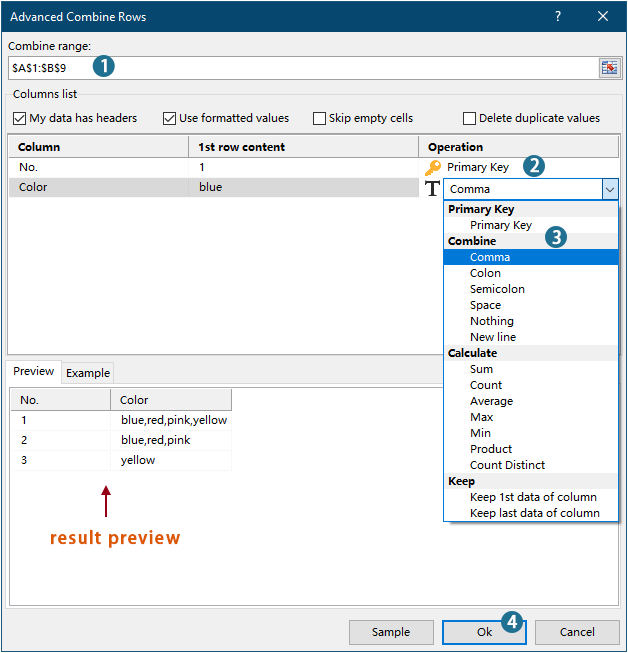
Yukarıda açıklanan yöntem, iki yardımcı sütun oluşturulmasını gerektirir ve uygunsuz olabilecek birden çok adım içerir. Daha basit bir yol arıyorsanız, kullanmayı düşünün. Gelişmiş Kombine Satırları aracı Kutools for Excel. Bu yardımcı program, yalnızca birkaç tıklamayla, belirli bir sınırlayıcı kullanarak hücreleri birleştirmenize olanak tanıyarak işlemi hızlı ve sorunsuz hale getirir.

Bahşiş: Bu aracı uygulamadan önce lütfen kurun Kutools for Excel birinci olarak. Şimdi ücretsiz indirmeye git.

1. tık Kutools > Birleştir ve Böl > Gelişmiş Kombine Satırları Bu özelliği etkinleştirmek için.
2. içinde Gelişmiş Kombine Satırları iletişim kutusunda yapmanız gerekenler:
  • Birleştirmek istediğiniz aralığı seçin;
  • ile aynı değerlere sahip sütunu ayarlayın. Birincil anahtar sütun.
  • Hücreleri birleştirmek için bir ayırıcı belirtin.
  • Tıkla OK.

Sonuç

not:

VBA kodu ile aynı değer varsa hücreleri birleştirin

Aynı değer başka bir sütunda varsa, bir sütundaki hücreleri birleştirmek için VBA kodunu da kullanabilirsiniz.

1. Basın Ara Toplam + F11 tuşlarını açmak için Microsoft Visual Basic Uygulamaları pencere.

2. içinde Microsoft Visual Basic Uygulamaları Pencere, tıklayın Ekle > modül. Ardından aşağıdaki kodu kopyalayıp modül pencere.

VBA kodu: aynı değerler varsa hücreleri birleştirin

Sub ConcatenateCellsIfSameValues()
	Dim xCol As New Collection
	Dim xSrc As Variant
	Dim xRes() As Variant
	Dim I As Long
	Dim J As Long
	Dim xRg As Range
	xSrc    = Range("A1", Cells(Rows.Count, "A").End(xlUp)).Resize(, 2)
	Set xRg = Range("D1")
	On Error Resume Next
	For I = 2 To UBound(xSrc)
		xCol.Add xSrc(I, 1), TypeName(xSrc(I, 1)) & CStr(xSrc(I, 1))
	Next I
	On Error GoTo 0
	ReDim xRes(1 To xCol.Count + 1, 1 To 2)
	xRes(1, 1) = "No"
	xRes(1, 2) = "Combined Color"
	For I = 1 To xCol.Count
		xRes(I + 1, 1) = xCol(I)
		For J = 2 To UBound(xSrc)
			If xSrc(J, 1) = xRes(I + 1, 1) Then
				xRes(I + 1, 2) = xRes(I + 1, 2) & ", " & xSrc(J, 2)
			End If
		Next J
		xRes(I + 1, 2) = Mid(xRes(I + 1, 2), 2)
	Next I
	Set xRg = xRg.Resize(UBound(xRes, 1), UBound(xRes, 2))
	xRg.NumberFormat = "@"
	xRg = xRes
	xRg.EntireColumn.AutoFit
End Sub

notlar:

1. D1 çizgide XRg = Aralık ("D1") ayarla sonucun D1 hücresinden başlayarak yerleştirileceği anlamına gelir.
2. "Yok hayır" ve "Kombine Renk" çizgide xRes (1, 1) = "Hayır" ve xRes (1, 2) = "Birleşik Renk" seçili sütunların başlıklarıdır. 

3. Tuşuna basın. F5 kodu çalıştırmak için tuşuna basın, ardından birleştirilmiş sonuçları belirtilen aralıkta alacaksınız.


Kutools for Excel ile aynı değerde hücreleri kolayca birleştirin

En İyi Ofis Üretkenlik Araçları

🤖 Kutools AI Yardımcısı: Aşağıdakilere dayalı olarak veri analizinde devrim yaratın: Akıllı Yürütme   |  Kodunu oluşturun  |  Özel Formüller Oluşturun  |  Verileri Analiz Edin ve Grafikler Oluşturun  |  Kutools İşlevlerini Çağır...
Popüler Özellikler: Yinelenenleri Bul, Vurgula veya Tanımla   |  Boş Satırları Sil   |  Veri Kaybı Olmadan Sütunları veya Hücreleri Birleştirin   |   Formülsüz Tur ...
Süper Arama: Çoklu Ölçütlü VLookup    Çoklu Değer VLookup  |   Birden Çok Sayfada VLookup   |   Bulanık Arama ....
Gelişmiş Açılır Liste: Hızla Açılır Liste Oluşturun   |  Bağımlı Açılır Liste   |  Çoklu Seçim Açılır Liste ....
Sütun Yöneticisi: Belirli Sayıda Sütun Ekleme  |  Sütunları Taşı  |  Gizli Sütunların Görünürlük Durumunu Değiştir  |  Aralıkları ve Sütunları Karşılaştırın ...
Öne Çıkan Özellikler: Izgara Odağı   |  Tasarım görünümü   |   Büyük Formül Çubuğu    Çalışma Kitabı ve Sayfa Yöneticisi   |  Kaynak Kütüphanesi (Otomatik metin)   |  Tarih Seçici   |  Çalışma Sayfalarını Birleştirin   |  Hücreleri Şifrele/Şifresini Çöz    E-postaları Listeye Göre Gönder   |  Süper Filtre   |   Özel Filtre (kalın/italik/üstü çizili filtre...) ...
En İyi 15 Araç Seti12 Metin Tools (Metin ekle, Karakterleri Kaldır, ...)   |   50+ Grafik Türleri (Gantt şeması, ...)   |   40+ Pratik Formüller (Yaşı doğum gününe göre hesapla, ...)   |   19 sokma Tools (QR Kodunu Girin, Yoldan Resim Ekle, ...)   |   12 Dönüştürme Tools (Sayılardan Kelimelere, Para Birimi Dönüştürme, ...)   |   7 Birleştir ve Böl Tools (Gelişmiş Kombine Satırları, Bölünmüş hücreler, ...)   |   ... ve dahası

Kutools for Excel ile Excel Becerilerinizi Güçlendirin ve Daha Önce Hiç Olmadığı Gibi Verimliliği Deneyimleyin. Kutools for Excel, Üretkenliği Artırmak ve Zamandan Tasarruf Etmek için 300'den Fazla Gelişmiş Özellik Sunar.  En Çok İhtiyacınız Olan Özelliği Almak İçin Buraya Tıklayın...

Açıklama


Office Tab, Office'e Sekmeli Arayüz Getirir ve İşinizi Çok Daha Kolay Hale Getirir

  • Word, Excel, PowerPoint'te sekmeli düzenlemeyi ve okumayı etkinleştirin, Publisher, Access, Visio ve Project.
  • Yeni pencereler yerine aynı pencerenin yeni sekmelerinde birden çok belge açın ve oluşturun.
  • Üretkenliğinizi% 50 artırır ve her gün sizin için yüzlerce fare tıklamasını azaltır!
Comments (23)
No ratings yet. Be the first to rate!
This comment was minimized by the moderator on the site
thank you very much, the VBA code works very well but I have a question that I can't solve.

NO Color
1 red
1 blue
1 red
1 yellow
2 red
2 yellow


in this case, in column B we have some duplicate colors related to the same number. How can I have an output that only return the values once?

I would like an output like this

NO Color
1 red, blue, yellow
2 red, yellow
This comment was minimized by the moderator on the site
Hi

The second method described in the post can help you solve this problem. After following the steps to specify the settings, checking the Delect Duplicate Values option will delete all duplicates in the combined results.
https://www.extendoffice.com/images/stories/comments/comment-picture-zxm/concatenate.png
This comment was minimized by the moderator on the site
Thank you so much for this formula! It saved hours of investigation! Fantastic work :)
This comment was minimized by the moderator on the site
Hi Crystal,

Thanks for your reply. I'll have to put my thinking hat on again...
Thank you
This comment was minimized by the moderator on the site
Hello, the macro above works great! Thank you. Is it anyway possible (I tried, but not successful) to amend it to concatenate column B (description) based on duplicates in column A (HS code) but also taking column C (origin) in the combination?
So description texts concatenate per HS code per origin.
Also column D(quantity) and column E(value) must be summed per HS code and origin.

A B C D E
HS CODE DESCRIPTION ORIGIN QUANTITY VALUE
5407420000 TWEED CN 10 € 150,00
5407420000 COTTON CN 15 € 250,00
5407420000 POLYESTER TW 5 € 130,00
5407420000 ORGANIC COTTON US 18 € 450,00
5407420000 COTTON US 23 € 780,00
5407420000 VELVET DELUXE CN 20 € 380,00
5407420000 COTTON CN 10 € 120,00
5806310000 TWEED JP 15 € 35,00
5806310000 POLYESTER AU 20 € 78,00
5806310000 TWEED AU 25 € 254,00
5806310000 POLYESTER SG 130 € 888,00
5806310000 COTTON EU 120 € 945,00
5806310000 COTTON FABRIC EU 10 € 80,00


Result shopuld be:

5407420000 TWEED, COTTON, VELVET DULUXE, COTTON, CN 55 € 900,00
5407420000 POLYESTER TW 5 € 130,00
5407420000 ORGANIC COTTON, COTTON US 41 € 1230,00
5806310000 TWEED JP 15 € 35,00
5806310000 POLYESTER, TWEED AU 45 € 332,00
5806310000 POLYESTER SG 130 € 888,00
5806310000 COTTON, COTTON FABRIC EU 130 € 1025,00

I hope this possible, thank you!
This comment was minimized by the moderator on the site
Hi Ivar,

Thank you for your comment. I am not able to solve this problem with VBA code yet. Sorry for that.
You can try if the last method can help.
This comment was minimized by the moderator on the site
Hello, how would the VBA code be adjusted if I want to combine cells in column M based on the duplicates in column A?
This comment was minimized by the moderator on the site
Hi Kristin,To combine cells in column M based on the duplicates in column A, try the VBA below.In the code,  O1 is the first cell to output the results; M is the column you will combine based on the duplicates in column A; A1 and A represent the first cell and the column where the duplicates locate; No and Combine color is the header of the columns after concatenating. You can change these variables as needed.<div data-tag="code">Sub ConcatenateCellsIfSameValues()
'Updated by Extendoffice 20211105
Dim xCol As New Collection
Dim xSrc As Variant
Dim xSrcValue As Variant
Dim xRes() As Variant
Dim I As Long
Dim J As Long
Dim xRg As Range
Dim xResultAddress As String
Dim xMergeAddress As String
Dim xUp As Integer

xResultAddress = "O1" 'The cell to output the results
xMergeAddress = "M" 'The column you will combine based on the duplicates in column A

xSrc = Range("A1", Cells(Rows.Count, "A").End(xlUp)).Resize(, 1)
xUp = Range("A1", Cells(Rows.Count, "A").End(xlUp)).Rows.Count
xSrcValue = Range(xMergeAddress & "1:" & xMergeAddress & xUp)

Set xRg = Range(xResultAddress)
On Error Resume Next
For I = 2 To UBound(xSrc)
xCol.Add xSrc(I, 1), TypeName(xSrc(I, 1)) & CStr(xSrc(I, 1))
Next I

On Error GoTo 0
ReDim xRes(1 To xCol.Count + 1, 1 To 2)
xRes(1, 1) = "No"
xRes(1, 2) = "Combined Color"
For I = 1 To xCol.Count
xRes(I + 1, 1) = xCol(I)
For J = 2 To UBound(xSrc)
If xSrc(J, 1) = xRes(I + 1, 1) Then
xRes(I + 1, 2) = xRes(I + 1, 2) & ", " & xSrcValue(J, 1)
End If
Next J
xRes(I + 1, 2) = Mid(xRes(I + 1, 2), 2)
Next I
Set xRg = xRg.Resize(UBound(xRes, 1), UBound(xRes, 2))
xRg.NumberFormat = "@"
xRg = xRes
xRg.EntireColumn.AutoFit
End Sub
This comment was minimized by the moderator on the site
I just wanted to thank you. It wasn't exactly what I wanted but man did it help me figure out what to do.

I have a table where the person's name was in column A, dates in column B and the names of tools they use in the headers of columns C:G . In each column there is a "Y" if they used that tool on that date and blank if they did not. (FYI: the same person can be listed more than once and may have used the same tool more than once) On a separate (summary) page I wanted to list all tools each person used within a date period, only listing each tool they used once, in the same cell. On this page, the person's name was in column A, Types of tools used in column B and the helper columns were in column G:K. Here's what I got:
The first helper column (G2):
=IF(COUNTIFS(Table7[Person's Name],A2,Table7[Screw Driver],"Y",Table7[Date],">="&1/1/20,Table7[Date],"<="&3/31/20),"Screw Driver","")
In the last helper column (K2):
=IF(COUNTIFS(Table7[Person's Name],A2,Table7[Hammer],"Y",Table7[Date],">="&1/1/20,Table7[Date],"<="&3/31/20),IF(J2="","Hammer",J2&"/"&"Hammer"),J2)

In B2 I just entered =K2

Thanks again and I hope this helps someone. EZPD
This comment was minimized by the moderator on the site
Hi, first of all thanks for creating this resource. I have been trying to figure this out for a couple of hours and I'm stuck. I'm using your 'concatenate cells if same value' but my script is looking at column "D" instead of "A. I can't figure out how to get it to use a different column for the data besides the one right next to it. In my cases I want it to look at column "D" to see if the value is the same and if so, it will grab the data from column "H" and put that data from column "H' into a cell in column "J". How do I switch this to use column "H" for the data? Thx


Sub ConcatenateCellsIfSameValues()
Dim xCol As New Collection
Dim xSrc As Variant
Dim xRes() As Variant
Dim I As Long
Dim J As Long
Dim xRg As Range
xSrc = Range("D1", Cells(Rows.Count, "D").End(xlUp)).Resize(, 2)
Set xRg = Range("J1")
On Error Resume Next
For I = 2 To UBound(xSrc)
xCol.Add xSrc(I, 1), TypeName(xSrc(I, 1)) & CStr(xSrc(I, 1))
Next I
On Error GoTo 0
ReDim xRes(1 To xCol.Count + 1, 1 To 2)
xRes(1, 1) = "No"
xRes(1, 2) = "Products"
For I = 1 To xCol.Count
xRes(I + 1, 1) = xCol(I)
For J = 2 To UBound(xSrc)
If xSrc(J, 1) = xRes(I + 1, 1) Then
xRes(I + 1, 2) = xRes(I + 1, 2) & vbCrLf & xSrc(J, 2)
End If
Next J
xRes(I + 1, 2) = Mid(xRes(I + 1, 2), 2)
Next I
Set xRg = xRg.Resize(UBound(xRes, 1), UBound(xRes, 2))
xRg.NumberFormat = "@"
xRg = xRes
xRg.EntireColumn.AutoFit
End Sub
This comment was minimized by the moderator on the site
"I can't figure out how to get it to use a different column for the data besides the one right next to it. In my cases I want it to look at column 'D' to see if the value is the same and if so, it will grab the data from column 'H' and put that data from column 'H' into a cell in column 'J'."

Did you ever figure this out?
This comment was minimized by the moderator on the site
Hi,

looks like 2 of your formulas are wrong :

=IF(A2<>A3,CONCATENATE(A2,",""",C2,""""),""). You need to change "A2" to "D1". As you'll want to add the string to the previous cell.

same goes for this formula :

=IF(A2<>A1,B2,C1 & "," & B2) : Change C1 to D1.


kind regards


Harry
This comment was minimized by the moderator on the site
I use this VBA for lots of my spreadsheets and its great. But the spreadsheets have become very large 50k+ rows and it doesnt seem to be working any more. If I use it on 1000 rows it works fine but large sets of data it cant seem to cope with. No errors just no results. Any help would be appreciated.
This comment was minimized by the moderator on the site
Hi James,
I tested the code as you mentioned, but it still works well in my case even I set the rows to 1000+.
This comment was minimized by the moderator on the site
Using the VBA macro and getting great results, I have tried tweaking it slightly for my needs but cant get it to work so I hope you can help.

Which bit do I change to make it concat a specific column, not the one directly to the right of the xSrc = Range?

Thanks for your great work!
This comment was minimized by the moderator on the site
Or as a better option, if you had 3 columns instead of 2 and found duplicates in column A (like your example) can you concat column B into a cell and column C into a seperate cell? So if you had columns of Number, Colour, Age, could you concat colour and age into different columns upon finding duplicates in Number? Hope that makes sense!
There are no comments posted here yet
Load More
Please leave your comments in English
Posting as Guest
×
Rate this post:
0   Characters
Suggested Locations