Excel'de birden fazla eşleşen değeri aramak (vlookup) ve birleştirmek nasıl yapılır?

Excel'de VLOOKUP kullanırken, işlev genellikle belirli bir arama kriteri için bulduğu ilk eşleşen değeri döndürür. Ancak, bir sınıftaki tüm öğrencileri listelemek veya belirli bir kategoriye ait tüm ürünleri listelemek gibi, belirli bir anahtarla ilişkili tüm eşleşen değerleri almanız ve birleştirmeniz gereken birçok yaygın senaryo vardır. Standart VLOOKUP işlevi bu konuda sınırlı olduğundan, hem arama yapmak hem de birden fazla eşleşen sonucu tek bir hücrede birleştirmek için nasıl bir çözüm bulunabileceğini merak edebilirsiniz. Aşağıda, farklı Excel sürümleri ve kullanıcı tercihlerine uygun olarak bu görevi gerçekleştirmek için çeşitli pratik ve verimli yöntemler ele alınacaktır.

Excel'de birden fazla eşleşen değeri arayın ve birleştirin

• TEXTJOIN ve FILTER İşlevlerini Kullanma (Excel365/2021)
• Kutools for Excel Kullanımı
• Kullanıcı Tanımlı İşlev Kullanımı
• Çoklu Birleştirme İçin VBA Kodu Kullanımı

TEXTJOIN ve FILTER İşlevleri ile Birden Fazla Eşleşen Değeri Ara ve Birleştir

Excel 365 veya Excel 2021 kullanıyorsanız, TEXTJOIN ve FILTER işlevlerinin kombinasyonu, tüm eşleşen değerleri aramak ve birleştirmek için etkili, formül tabanlı bir yaklaşım sunar. Bu çözüm özellikle dinamik ve güncellenen veri setleri için uygundur, çünkü kaynak veriler değiştiğinde sonuç otomatik olarak yenilenir. En iyi şekilde, FILTER fonksiyonunu destekleyen Excel sürümlerinde uygulanır; bu özellik yalnızca son Office sürümlerinde mevcuttur.

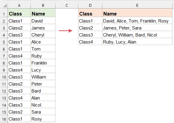
Hedef hücreye aşağıdaki formülü girin, ardından formülü diğer satırlara da uygulamak istiyorsanız aşağı doğru sürükleyin. Tüm eşleşen değerler çıkarılır ve tek bir hücrede birleştirilir. Ekran görüntüsüne bakın:

=TEXTJOIN(", ", TRUE, FILTER($B$2:$B$16, $A$2:$A$16=D2, ""))

Kutools for Excel ile birden fazla eşleşen değeri ara ve birleştir

Yerleşik formül yöntemlerini zor buluyorsanız veya Excel sürümünüz TEXTJOIN ve FILTER gibi gelişmiş işlevleri desteklemiyorsa, Kutools for Excel kullanıcı dostu bir grafiksel çözüm sunar. Kutools'un Birçoklu Arama özelliği, birkaç adımda birden fazla eşleşen sonucu aramanıza ve birleştirmenize olanak tanır; bu hem başlangıç seviyesindeki hem de ileri düzeydeki kullanıcılar için uygundur. Kutools ile karmaşık formüller veya kodlar yazmanıza gerek yoktur ve özellikle tekrarlayan aramalar ve toplamalar gerektiren büyük veya değişken veri setleriyle çalışırken elverişlidir.

Kutools for Excel'i yükledikten sonra aşağıdaki adımları izleyin:

Kutools > Süper ARA > Birçoklu arama (birden fazla sonuç döndürme) öğesine tıklayarak kurulum iletişim kutusunu açın. Bu iletişim kutusu içinde, aşağıdaki adımları kullanarak arama ve çıktı ayarlarınızı hızlıca yapılandırabilirsiniz:

1. Birleştirilmiş sonuçlar için hedef çıktı hücrelerini ve aramak istediğiniz değerleri içeren hücreleri seçin;
2. Arama anahtarı ve sonuç sütunlarını içeren tablo aralığını belirtin;
3. Hangi sütunun arama anahtarlarını içerdiğini (Anahtar Sütun) ve hangi sütunun değerlerinin birleştirileceğini (Dönüş Sütunu) belirtin;
4. Ayarlarınızı onaylamak ve verileri işlemek için Tamam düğmesine tıklayın.
   

Sonuç: Kutools, seçtiğiniz çıktı hücresinde tüm eşleşen ve birleştirilmiş değerleri görüntüleyecektir. Ekran görüntüsüne bakın:

Bu yöntem, karmaşık formüller veya kodlar olmadan doğrudan Excel arabiriminden çalışmayı tercih edenler için oldukça tavsiye edilir. Ayrıca, formül hatalarının olasılığını azaltır ve tekrarlayan arama ve birleştirme görevlerinde üretkenliği artırır.

Kullanıcı Tanımlı İşlev ile birden fazla eşleşen değeri ara ve birleştir

VBA (Visual Basic for Applications) ile yetkin olan veya dinamik dizi veya FILTER işlev desteği olmayan eski Excel sürümlerini kullanan kullanıcılar için, esnek bir çoklu sonuç birleştirme özelliği sağlayan özel bir Kullanıcı Tanımlı İşlev (UDF) oluşturabilirsiniz. Bu yöntem tüm Excel sürümleriyle tamamen uyumludur ve belirli ayırıcı semboller veya koşullara göre özelleştirilebilir.

1. ALT + F11 tuşlarına basılı tutarak Microsoft Visual Basic for Applications penceresini açın.

2. Ekle > Modül'e tıklayın ve aşağıdaki kodu Modül Penceresine yapıştırın.

VBA kodu: Bir hücrede birden fazla eşleşen değeri ara ve birleştir

Function ConcatenateMatches(LookupValue As String, LookupRange As Range, ReturnRange As Range, Optional Delimiter As String = ", ") As String
'Updateby Extendoffice
    Dim Cell As Range
    Dim Result As String
    Result = ""
    For Each Cell In LookupRange
        If Cell.Value = LookupValue Then
            Result = Result & Cell.Offset(0, ReturnRange.Column - LookupRange.Column).Value & Delimiter
        End If
    Next Cell
    If Result <> "" Then
        Result = Left(Result, Len(Result) - Len(Delimiter))
    End If
    ConcatenateMatches = Result
End Function

3. VBA düzenleyicisini kaydedip kapatın. Çalışma sayfanıza dönün ve bu UDF'yi şu formülü kullanarak uygulayın: =ConcatenateMatches(D2, $A$2:$A$16, $B$2:$B$16) , istediğiniz sonucu almak istediğiniz boş bir hücreye girin. Gerekirse formülü diğer hücrelere kopyalamak için doldurma tutamacını aşağı doğru sürükleyin. Belirli bir arama değerine dayalı olarak tüm eşleşen değerler döndürülür ve virgül ve boşlukla ayrılmış tek bir hücrede birleştirilir. Ekran görüntüsüne bakın:

VBA kodu ile birden fazla eşleşen değeri ara ve birleştir

Tekrarlayan kullanım gerektiren senaryolar için veya çalışma sayfası hücrelerinde özel işlevlerden kaçınmak isteyenler için, sonuçları doğrudan birleştirmek üzere hazır bir VBA makrosu kullanabilirsiniz. Bu yöntem, tüm kullanıcıların aynı sürüm veya eklentilere sahip olmadığı ortak ortamlarda iyi çalışır.

1. Geliştirici Araçları > Visual Basic'e tıklayarak VBA düzenleyicisini açın.

2. VBA penceresinde Ekle > Modül'e tıklayın, ardından bu kodu modüle yapıştırın:

Sub VLookupAndConcatenate()
    Dim ws As Worksheet
    Dim dataRange As Range, lookupRange As Range, resultRange As Range
    Dim dict As Object
    Dim i As Long, lastRow As Long
    Dim lookupValue As Variant, result As String
    Dim delimiter As String
    delimiter = ", "
    Set dict = CreateObject("Scripting.Dictionary")
    Set ws = ActiveSheet
    On Error Resume Next
    Set dataRange = Application.InputBox( _
        Prompt:="Please select the data range (contains lookup column and result column)", _
        Title:="Select Data Range", _
        Type:=8)
    On Error GoTo 0
    If dataRange Is Nothing Then Exit Sub
    On Error Resume Next
    Set lookupRange = Application.InputBox( _
        Prompt:="Please select the lookup range (single column)", _
        Title:="Select Lookup Range", _
        Type:=8)
    On Error GoTo 0
    If lookupRange Is Nothing Then Exit Sub
    On Error Resume Next
    Set resultRange = Application.InputBox( _
        Prompt:="Please select the starting cell for results output", _
        Title:="Select Output Location", _
        Type:=8)
    On Error GoTo 0
    If resultRange Is Nothing Then Exit Sub
    resultRange.Resize(lookupRange.Rows.Count, 1).ClearContents
    For i = 1 To dataRange.Rows.Count
        lookupValue = dataRange.Cells(i, 1).Value
        If Not dict.Exists(lookupValue) Then
            dict.Add lookupValue, dataRange.Cells(i, 2).Value
        Else
            dict(lookupValue) = dict(lookupValue) & delimiter & dataRange.Cells(i, 2).Value
        End If
    Next i
    For i = 1 To lookupRange.Rows.Count
        lookupValue = lookupRange.Cells(i, 1).Value
        If dict.Exists(lookupValue) Then
            resultRange.Cells(i, 1).Value = dict(lookupValue)
        Else
            resultRange.Cells(i, 1).Value = "Not Found"
        End If
    Next i
    MsgBox "Operation completed! Processed " & lookupRange.Rows.Count & " lookup values.", vbInformation
End Sub

3. Tıklayın düğmesine basarak makroyu çalıştırın. Giriş kutuları, veri aralığınızı, arama aralığınızı ve sonuç aralığınızı seçmenizi isteyecektir. Birleştirilmiş sonuç daha sonra seçilen çıktı hücrelerinde doğrudan görüntülenir.

Bu makro yaklaşımı, özellikle farklı değerlerle çoklu birleştirme aramaları sıkça gerçekleştirdiğiniz durumlarda faydalıdır, çünkü çalışma sayfasını UDF çağrılarıyla karıştırmaktan kaçınır.

Gerektiğinde kodda ayırıcıyı kolayca ayarlayabilir ve makroyu iş akışınıza göre sonuçları bir hücreye veya dosyaya çıkarmak için genişletebilirsiniz.

Excel'de birden fazla eşleşen değeri birleştirmek, durumunuza bağlı olarak belirli avantajlara sahip çeşitli yaklaşımlar kullanılarak mümkündür. Dinamik dizi formülleri, Kutools for Excel gibi eklentiler veya VBA tabanlı yöntemler arasından seçim yaparak gruplandırılmış verileri analiz etme ve görüntüleme yeteneğinizi geliştireceksiniz. Veri setinizin boyutuna ve karmaşıklığına bağlı olarak, kendiniz veya takımınız için en uygun performansı ve bakım kolaylığını sağlayan yaklaşımı değerlendirin. Günlük işlemlerde, veri tutarlılığını kontrol edin, birleştirilmiş hücrelerden kaçının ve en iyi sonuçlar için referans aralıklarını doğrulayın. Formül hesaplamalarında hata karşılaşırsanız, aralıkların verilerle eşleştiğinden ve Excel sürümünüz için doğru formül giriş yöntemini kullandığınızdan emin olun.

Daha gelişmiş Excel teknikleri ve çeşitli pratik nasıl yapılır kılavuzları için kapsamlı eğitim kütüphanemizi ziyaret edin.