Bir hücre Excel'de belirli bir metin içeriyorsa, başka bir hücrede değer nasıl döndürülür?

Aşağıda gösterilen örnekte olduğu gibi, E6 hücresi "Evet" değerini içerdiğinde, F6 hücresi otomatik olarak "onayla" değeriyle doldurulacaktır. E6'da "Evet"i "Hayır" veya "Tarafsızlık" olarak değiştirirseniz, F6'daki değer hemen "Reddet" veya "Yeniden Düşün" olarak değiştirilir. Bunu başarmak için nasıl yapabilirsiniz? Bu makale, kolayca çözmenize yardımcı olacak bazı yararlı yöntemler toplar.

Bir hücre formül içeren belirli bir metin içeriyorsa, başka bir hücrede dönüş değeri

Bir hücre yalnızca belirli bir metin içeriyorsa, başka bir hücrede değer döndürmek için lütfen aşağıdaki formülü deneyin. Örneğin, B5 "Evet" içeriyorsa, D5'te "Onayla" döndür, aksi takdirde "Nitelikli değil" döndür. Lütfen aşağıdaki gibi yapın.

D5'i seçin ve aşağıdaki formülü içine kopyalayın ve Keşfet anahtar. Ekran görüntüsüne bakın:

Hücre, formüle sahip farklı metinler içeriyorsa, değerleri başka bir hücrede döndür

Bu bölüm, bir hücre Excel'de farklı metin içeriyorsa, başka bir hücrede değerleri döndürmenin formülünü gösterecektir.

1. İki sütunda ayrı ayrı bulunan belirli değerler ve dönüş değerleri ile bir tablo oluşturmanız gerekir. Ekran görüntüsüne bakın:

2. Değeri döndürmek için boş bir hücre seçin, içine aşağıdaki formülü yazın ve Keşfet sonucu almak için anahtar. Ekran görüntüsüne bakın:

Şu andan itibaren, E6'daki değeri belirli bir değerle değiştirirken, karşılık gelen değeri hemen F6'da döndürülecektir.

Bir hücre farklı metinler içeriyorsa, değerleri başka bir hücrede kolayca döndürün

Aslında yukarıdaki sorunu daha kolay bir şekilde çözebilirsiniz. Listede bir değer arayın yarar Kutools for Excel formülü hatırlamadan sadece birkaç tıklama ile başarmanıza yardımcı olabilir.

1. Yukarıdaki yöntemle aynı şekilde, iki sütunda ayrı ayrı bulunan belirli değerler ve dönüş değerleri ile bir tablo oluşturmanız da gerekir.

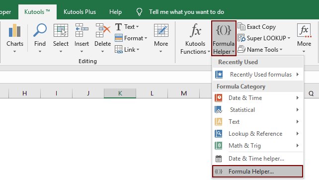
2. Sonucun çıktısını almak için boş bir hücre seçin (burada F6'yı seçiyorum) ve ardından Kutools > Formül Yardımcısı > Formül Yardımcısı. Ekran görüntüsüne bakın:

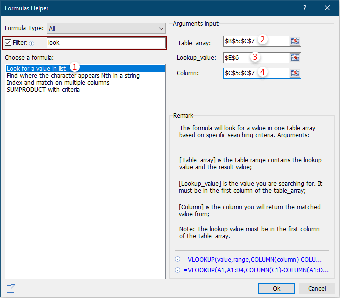
3. içinde Formül Yardımcısı iletişim kutusu, lütfen aşağıdaki gibi yapılandırın:

• 3.1 içinde Bir formül seçin kutusu bul ve seç Listede bir değer arayın;
  İpuçları: Kontrol edebilirsiniz filtre kutusunda, formülü hızla filtrelemek için metin kutusuna belirli bir kelimeyi girin.
• 3.2 içinde Masa dizisi kutusunda, 1. adımda oluşturduğunuz başlıkların olmadığı tabloyu seçin;
• 3.2 içinde aranan_değer kutusunda, hücreye dayalı olarak değer döndüreceğiniz belirli değeri içerir;
• 3.3 içinde Sütun kutusunda eşleşen değeri döndüreceğiniz sütunu belirtin. Veya sütun numarasını ihtiyaç duyduğunuzda doğrudan metin kutusuna girebilirsiniz.
• 3.4 OK buton. Ekran görüntüsüne bakın:

Şu andan itibaren, E6'daki değeri belirli bir değerle değiştirirken, karşılık gelen değeri hemen F6'da döndürülecektir. Aşağıdaki gibi sonucu görün:

Excel için Kutools - Her Zaman Zamanının Ötesinde Çalışmanızı Bitirmenize, Hayatın Keyfini Çıkarmak için Daha Fazla Zamana Sahip Olmanıza Yardımcı

Kendinizi sık sık işe yetişirken, kendinize ve ailenize harcayacak zamanın olmadığını mı buluyorsunuz?  Kutools for Excel başa çıkmanıza yardımcı olabilir %80 Excel bulmacaları ve iş verimliliğini %80 artırın, size ailenizle ilgilenmek ve hayatın tadını çıkarmak için daha fazla zaman verin.

300 çalışma senaryosu için 1500 gelişmiş araç, işinizi her zamankinden çok daha kolay hale getirir.
Artık formülleri ve VBA kodlarını ezberlemenize gerek yok, bundan sonra beyninizi dinlendirin.
Karmaşık ve tekrarlanan işlemler, saniyeler içinde tek seferlik bir işlem yapılabilir.
Her gün binlerce klavye ve fare işlemini azaltın, meslek hastalıklarına şimdi veda edin.
3 dakika içinde Excel uzmanı olun, hızlı bir şekilde tanınmanıza ve maaş zammı promosyonuna yardımcı olun.
110,000 son derece etkili insan ve 300'den fazla dünyaca ünlü şirketin seçimi.
39.0 $ 'lık değeri 4000.0 $' dan fazla olan başkalarının eğitimini yapın.
30 günlük tam özellikli ücretsiz deneme. Sebepsiz 60 Günlük Para İade Garantisi.