Excel'de en yüksek puanın karşılık gelen adını nasıl görüntülersiniz?
Diyelim ki, iki sütun içeren bir veri aralığım var – isim sütunu ve buna karşılık gelen puan sütunu, şimdi en yüksek puan alan kişinin adını almak istiyorum. Bu sorunu Excel'de hızlı bir şekilde çözmek için herhangi iyi yöntemler var mı?
En yüksek puanın karşılık gelen adını formüllerle görüntüleme
 En yüksek puanın karşılık gelen adını formüllerle görüntüleme
En yüksek puanı alan kişinin adını almak için aşağıdaki formüller size sonucu elde etmenize yardımcı olabilir.
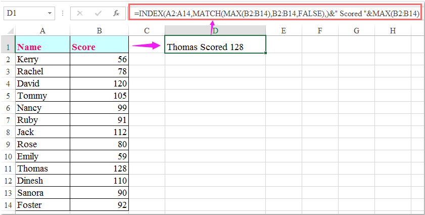
Lütfen bu formülü girin: =INDEX(A2:A14,MATCH(MAX(B2:B14),B2:B14,YANLIŞ),)&" Skor "&MAX(B2:B14) adı görüntülemek istediğiniz boş bir hücreye yazın ve ardından Enter tuşuna basarak aşağıdaki gibi sonucu alın:
Notlar:
1. Yukarıdaki formülde A2:A14, ad almak istediğiniz listedir ve B2:B14 puan listesidir.
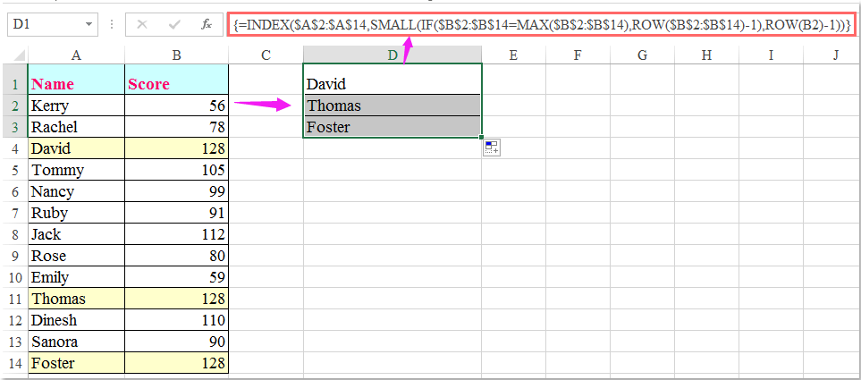
2. Yukarıdaki formül, birden fazla aynı en yüksek puana sahip isim varsa yalnızca ilk ismi alabilir. En yüksek puanı alan tüm isimleri almak için aşağıdaki dizi formülü işinize yarayabilir.
Bu formülü girin:
=INDEX($A$2:$A$14,SMALL(IF($B$2:$B$14=MAX($B$2:$B$14),ROW($B$2:$B$14)-1),ROW(B2)-1)), ardından Ctrl + Shift + Enter tuşlarına birlikte basarak ilk ismi görüntüleyin, sonra formül hücresini seçin ve doldurma tutamacını aşağı doğru sürükleyin, hata değeri görünene kadar en yüksek puanı alan tüm isimler aşağıdaki ekran görüntüsünde gösterildiği gibi görüntülenir:

Kutools AI ile Excel Sihirini Keşfedin
- Akıllı Yürütme: Hücre işlemleri gerçekleştirin, verileri analiz edin ve grafikler oluşturun—tümü basit komutlarla sürülür.
- Özel Formüller: İş akışlarınızı hızlandırmak için özel formüller oluşturun.
- VBA Kodlama: VBA kodunu kolayca yazın ve uygulayın.
- Formül Yorumlama: Karmaşık formülleri kolayca anlayın.
- Metin Çevirisi: Elektronik tablolarınız içindeki dil engellerini aşın.
En İyi Ofis Verimlilik Araçları
Kutools for Excel ile Excel becerilerinizi güçlendirin ve benzersiz bir verimlilik deneyimi yaşayın. Kutools for Excel, üretkenliği artırmak ve zamandan tasarruf etmek için300'den fazla Gelişmiş Özellik sunuyor. İhtiyacınız olan özelliği almak için buraya tıklayın...
Office Tab, Ofis uygulamalarına sekmeli arayüz kazandırır ve işinizi çok daha kolaylaştırır.
- Word, Excel, PowerPoint'te sekmeli düzenleme ve okuma işlevini etkinleştirin.
- Yeni pencereler yerine aynı pencerede yeni sekmelerde birden fazla belge açıp oluşturun.
- Verimliliğinizi %50 artırır ve her gün yüzlerce mouse tıklaması azaltır!
Tüm Kutools eklentileri. Tek kurulum
Kutools for Office paketi, Excel, Word, Outlook & PowerPoint için eklentileri ve Office Tab Pro'yu bir araya getirir; Office uygulamalarında çalışan ekipler için ideal bir çözümdür.
- Hepsi bir arada paket — Excel, Word, Outlook & PowerPoint eklentileri + Office Tab Pro
- Tek kurulum, tek lisans — dakikalar içinde kurulun (MSI hazır)
- Birlikte daha verimli — Ofis uygulamalarında hızlı üretkenlik
- 30 günlük tam özellikli deneme — kayıt yok, kredi kartı yok
- En iyi değer — tek tek eklenti almak yerine tasarruf edin