Açılır listede boş yerine ilk öğeyi nasıl gösteririz?
Excel çalışma sayfalarındaki açılır listeler, veri girişi sürecini hızlandırmak ve standartlaştırmak için pratik bir özelliktir—kullanıcılar değerleri tek tek yazmak yerine önceden tanımlanmış seçenekler arasından seçim yapabilir. Ancak bazen, bir açılır hücreye tıkladığınızda ilk seçimin boş olarak göründüğü durumlarla karşılaşabilirsiniz; bu da listenin gerçek ilk veri öğesi yerine boşluk gösterilmesinden kaynaklanır. Bu sorun genellikle kaynak veri listesi düzenlendiğinde ve sonunda boş satırlar kaldığında veya listenin sonundaki öğeler silindiğinde ortaya çıkar. Özellikle uzun listelerde, sürekli olarak boş girişlerden geçip ilk geçerli öğeye ulaşmak zaman alıcı ve sinir bozucu olabilir.

Bu sorunu çözmek sadece kullanıcılar için kolaylık sağlayacak, aynı zamanda sonraki veri işleme veya raporlama görevlerini etkileyebilecek boş değerlerin yanlışlıkla seçilmesini de engelleyecektir. Bu makalede, açılır listenizin ilk girdisinin her zaman en üstte görünmesini sağlamak için pratik yöntemler öğreneceksiniz; böylece bu gereksiz boşluklar ortadan kalkmış olacak.
Veri Doğrulama işlevi ile boş yerine açılır listedeki ilk öğeyi gösterme
VBA kodu ile boş yerine açılır listedeki ilk öğeyi otomatik olarak gösterme
Veri Kaynağı Olarak Excel Tablosu Kullanımı
Veri Doğrulama işlevi ile boş yerine açılır listedeki ilk öğeyi gösterme
Açılır listenizin başında boş girişleri önlemek için etkili bir yöntem, doğru aralığı dinamik olarak belirleyen bir formül kullanarak Veri Doğrulama ayarını yapmaktır. Bu yaklaşım, listenin sonundaki verilerin silinmesi nedeniyle oluşan boş satırlardan bağımsız olarak, yalnızca kaynak listenizdeki dolu hücrelerin dahil edilmesini sağlar. Bu çözüm özellikle kaynak listeyi sık sık değiştiren veya makro kullanmadan basit bir formül tabanlı düzenleme yapmak isteyen kullanıcılar için uygundur.
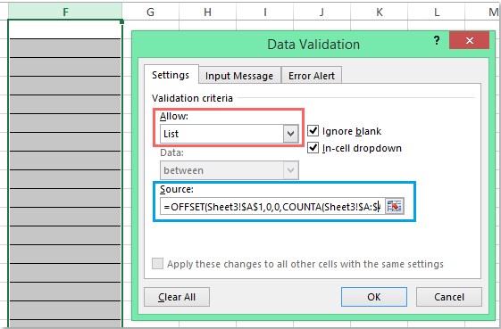
1. Açılır liste oluşturmak istediğiniz hücreleri seçin. Ardından, Excel şeridine gidin ve Veri > Veri Doğrulaması > Veri Doğrulaması'na tıklayın. Aşağıda gösterildiği gibi Veri Doğrulama iletişim kutusu açılacaktır:

2. Veri Doğrulama iletişim kutusundaki Ayarlar sekmesinde İzin Ver'i Liste olarak ayarlayın. Kaynak kutusuna, yalnızca gerçek veri içeren aralığı dinamik olarak referans almak için şu formülü girin:
=OFFSET(Sheet3!$A$1,0,0,COUNTA(Sheet3!$A:$A)-1,1)
Not: Bu formülde, Sheet3 kaynak verilerinizin bulunduğu sayfayı ifade eder ve A1 listenizin başlangıç hücresidir. Bunları çalışma sayfanızın düzenine göre gerektiği gibi ayarlayın. COUNTA'nın kullanılması, yalnızca boş olmayan hücrelerin A1'den başlayarak dahil edilmesini sağlar. Kaynak listenizde kasıtlı boş satırlar varsa (yalnızca sonunda değil), bu yöntem onları tamamen hariç tutmayabilir, bu nedenle en iyi sonuçlar için kaynak listenizi bitişik tutun.
3. Ayarları uygulamak için Tamam'a tıklayın. Artık yapılandırdığınız açılır liste hücrelerinden herhangi birine tıkladığınızda, liste en üstte gerçek ilk veri öğesiyle görüntülenecektir. Bu, kaynak veriler değişse bile, A sütunundaki tüm öğeleri kapsayan bir aralık olduğu sürece ve ana veri bloğunuzda boş hücreler olmadığı müddetçe geçerli olacaktır. Aşağıdaki sonucu inceleyin:

İpucu: Daha sonra kaynak listenizi genişletmeniz veya daraltmanız gerekiyorsa, veri doğrulama ayarlarınızı güncellemeniz gerekmez. Formül, aralığınızın başında boş hücre olmadığı sürece otomatik olarak ayarlanır. Ancak, listede (yalnızca sonunda değil) bir boşluk varsa, hesaplama sayısında atlanır ancak açılır listede istenmeyen boşluklar oluşturabilir.
Olası sorun: Kaynak verilerinizde kasıtlı boşluklar varsa veya birleştirilmiş hücreleriniz veya bitişik olmayan verileriniz varsa, kaynak aralığınız olarak bir Excel Tablosu kullanmayı düşünün veya daha esnek bir işlem için aşağıdaki VBA yöntemini inceleyin.
VBA kodu ile boş yerine açılır listedeki ilk öğeyi otomatik olarak gösterme
Bazı senaryolarda, yalnızca veri doğrulama kaynağını ayarlamak yeterli olmayabilir—örneğin, verileriniz sık sık değişiyorsa veya kaynak aralığınızda başka yapısal nedenlerle boşluklar oluşma riski varsa. Basit bir VBA kodu ile, veri doğrulaması olan bir hücre her etkinleştirildiğinde açılır listede her zaman ilk mevcut öğenin otomatik olarak seçilmesini ve gösterilmesini sağlayabilirsiniz. Bu aynı zamanda kullanıcı tıklamalarını minimize ederek veri giriş hızını artırabilir.
1. Açılır listenizi ekledikten sonra, açılır listeyi içeren sayfa sekmesine sağ tıklayın ve bağlam menüsünden Kodu Görüntüle'yi seçin. Microsoft Visual Basic for Applications düzenleyicisi açılacaktır. Pencerede, aşağıdaki kodu ilgili çalışma sayfası modülüne (standart modül değil) yapıştırın. Bu kod, arka planda çalışır ve bir doğrulama hücresi seçtiğinizde her seferinde açılır listeyi sıfırlar:
VBA kodu: Açılır listedeki ilk veri öğesini otomatik olarak göster:
Private Sub Worksheet_SelectionChange(ByVal Target As Range)
'Updateby Extendoffice 20160725
    Dim xFormula As String
    On Error GoTo Out:
    xFormula = Target.Cells(1).Validation.Formula1
    If Left(xFormula, 1) = "=" Then
        Target.Cells(1) = Range(Mid(xFormula, 1)).Cells(1).Value
    End If
Out:
End Sub

2. Kodu yapıştırdıktan sonra, çalışma kitabınızı kaydedin (tercihen .xlsm uzantılı makro etkin dosya olarak) ve VBA düzenleyici penceresini kapatın. Şimdi, sayfanıza dönün ve açılır listeye sahip herhangi bir hücreye tıklayın—hücreyi etkinleştirdiğinizde, açılır listenizin ilk girdisi otomatik olarak görüntülenecektir.
İpuçları ve dikkat edilmesi gereken noktalar: Bu VBA yaklaşımı, özellikle dinamik veya uzun kaynak listeleri olan ya da kaçınılmaz boş girişler içeren listelerde kullanıcılar için sorunsuz bir deneyim istediğinizde idealdir. Bunu çalıştırmak için makroları etkinleştirmeyi unutmayın ve diğer kullanıcıları bilgilendirin, çünkü bazı ortamlar güvenlik nedeniyle makro kullanımını kısıtlayabilir.
Sorun giderme: Kod çalışmıyorsa, VBA düzenleyicisinde doğru çalışma sayfası kod penceresine yerleştirildiğinden emin olun. Ayrıca, açılır listenin standart bir Veri Doğrulama listesi kullandığından emin olun.
Sınırlama: VBA çözümü, kullanıcı açılır hücreyi seçtiğinde tetiklenecektir; hücre başka yollarla doldurulursa (örneğin, formül sonuçları veya yapıştırma yoluyla) çalışmaz. Hücreden açılır listeyi kaldırırsanız veya VBA kodu olmadan hücreyi başka bir sayfaya taşırsanız, otomatik seçim davranışı kaybolur.
Veri Kaynağı Olarak Excel Tablosu Kullanımı
Açılır listenizin kaynak listesi dinamikse ve daha iyi bakım yapılmasını istiyorsanız, kaynak listenizi bir Excel Tablosuna dönüştürmeyi düşünün. Tablolar, veri eklendiğinde veya kaldırıldığında boyutlarını otomatik olarak ayarlar, bu nedenle listeniz güncel kalır. Ancak, bir Excel Tablosu boş hücreleri otomatik olarak hariç tutmaz—tablodaki boş girişler hala açılır listede görünecektir, bunları açıkça filtrelemediğiniz sürece (örneğin, Excel 365 ve Excel 2021'de bulunan FİLTRE fonksiyonunu kullanarak).
1. Kaynak verilerinizi seçin ve Ctrl + T tuşlarına basarak bir Tablo'ya dönüştürün. En üstte boşluk olmadığından emin olun. Tabloya Anlamlı bir isim verin, örneğin MyList (Tablo Tasarımı sekmesini kullanarak).
2. Veri doğrulaması ayarlarını yaparken, tablo sütununa yapılandırılmış referansı kullanın. Veri Doğrulaması'nın Kaynak kısmına şunu yazın:
=INDIRECT("MyList[Column1]")Column1'i gerçek sütun adınızla değiştirin (sütun başlığı). Bu yöntem, tablo sütunundaki tüm dolu öğeleri dinamik olarak içerir ve verileri güncelledikçe listenin bütünlüğünü korur.
Bu yaklaşım özellikle kaynak verilerin düzenli olarak güncellendiği ve birden fazla kullanıcının doğrulanmış listeyi etkili bir şekilde yönetmesi gereken ortamlar için uygundur.
En İyi Ofis Verimlilik Araçları
Kutools for Excel ile Excel becerilerinizi güçlendirin ve benzersiz bir verimlilik deneyimi yaşayın. Kutools for Excel, üretkenliği artırmak ve zamandan tasarruf etmek için300'den fazla Gelişmiş Özellik sunuyor. İhtiyacınız olan özelliği almak için buraya tıklayın...
Office Tab, Ofis uygulamalarına sekmeli arayüz kazandırır ve işinizi çok daha kolaylaştırır.
- Word, Excel, PowerPoint'te sekmeli düzenleme ve okuma işlevini etkinleştirin.
- Yeni pencereler yerine aynı pencerede yeni sekmelerde birden fazla belge açıp oluşturun.
- Verimliliğinizi %50 artırır ve her gün yüzlerce mouse tıklaması azaltır!
Tüm Kutools eklentileri. Tek kurulum
Kutools for Office paketi, Excel, Word, Outlook & PowerPoint için eklentileri ve Office Tab Pro'yu bir araya getirir; Office uygulamalarında çalışan ekipler için ideal bir çözümdür.
- Hepsi bir arada paket — Excel, Word, Outlook & PowerPoint eklentileri + Office Tab Pro
- Tek kurulum, tek lisans — dakikalar içinde kurulun (MSI hazır)
- Birlikte daha verimli — Ofis uygulamalarında hızlı üretkenlik
- 30 günlük tam özellikli deneme — kayıt yok, kredi kartı yok
- En iyi değer — tek tek eklenti almak yerine tasarruf edin