Excel'de n'inci boş olmayan hücreyi nasıl bulurum?
Excel'deki bir sütun veya satırdan n'inci boş olmayan hücre değerini nasıl bulabilir ve döndürebilirsiniz? Bu makalede, size bu görevi çözmeye yardımcı olacak bazı yararlı formüller tartışacağım.
Formülle bir sütundan n'inci boş olmayan hücre değerini bulma ve döndürme
Formülle bir satırdan n'inci boş olmayan hücre değerini bulma ve döndürme
 Formülle bir sütundan n'inci boş olmayan hücre değerini bulma ve döndürme
Örneğin, aşağıdaki ekran görüntüsünde gösterildiği gibi bir sütun verim var, şimdi bu listeden üçüncü boş olmayan hücre değerini alacağım.
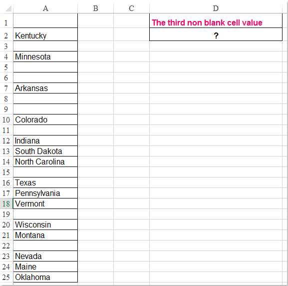
Lütfen bu formülü: =INDEX($A$1:$A$25,SMALL(ROW($A$1:$A$25)+(100*($A$1:$A$25="")), 3))&"" sonucu çıkarmak istediğiniz boş bir hücreye girin, örneğin D2 ve ardından doğru sonucu elde etmek için Ctrl + Shift + Enter tuşlarına birlikte basın, ekran görüntüsüne bakın:

Not: Yukarıdaki formülde, A1:A25 kullanmak istediğiniz veri listesidir ve 3 sayısı döndürmek istediğiniz üçüncü boş olmayan hücre değerini belirtir. İkinci boş olmayan hücreyi almak istiyorsanız, gerekli şekilde 3 sayısını 2 olarak değiştirin.
Formülle bir satırdan n'inci boş olmayan hücre değerini bulma ve döndürme
Bir satırdaki n'inci boş olmayan hücre değerini bulmak ve döndürmek istiyorsanız, aşağıdaki formül size yardımcı olabilir, lütfen şu adımları izleyin:
Bu formülü girin: =INDEX($A$1:$M$1,SMALL(IF($A$1:$M$1<>"",COLUMN($A$1:$M$1)-COLUMN($A$1)+1),4)) sonucu yerleştirmek istediğiniz boş bir hücreye yazın ve ardından sonucu elde etmek için Ctrl + Shift + Enter tuşlarına birlikte basın, ekran görüntüsüne bakın:
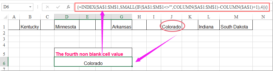
Not: Yukarıdaki formülde, A1:M1 kullanmak istediğiniz satır değerleridir ve 4 sayısı döndürmek istediğiniz dördüncü boş olmayan hücre değerini belirtir. İkinci boş olmayan hücreyi almak istiyorsanız, gerekli şekilde 4 sayısını 2 olarak değiştirin.
En İyi Ofis Verimlilik Araçları
Kutools for Excel ile Excel becerilerinizi güçlendirin ve benzersiz bir verimlilik deneyimi yaşayın. Kutools for Excel, üretkenliği artırmak ve zamandan tasarruf etmek için300'den fazla Gelişmiş Özellik sunuyor. İhtiyacınız olan özelliği almak için buraya tıklayın...
Office Tab, Ofis uygulamalarına sekmeli arayüz kazandırır ve işinizi çok daha kolaylaştırır.
- Word, Excel, PowerPoint'te sekmeli düzenleme ve okuma işlevini etkinleştirin.
- Yeni pencereler yerine aynı pencerede yeni sekmelerde birden fazla belge açıp oluşturun.
- Verimliliğinizi %50 artırır ve her gün yüzlerce mouse tıklaması azaltır!
Tüm Kutools eklentileri. Tek kurulum
Kutools for Office paketi, Excel, Word, Outlook & PowerPoint için eklentileri ve Office Tab Pro'yu bir araya getirir; Office uygulamalarında çalışan ekipler için ideal bir çözümdür.
- Hepsi bir arada paket — Excel, Word, Outlook & PowerPoint eklentileri + Office Tab Pro
- Tek kurulum, tek lisans — dakikalar içinde kurulun (MSI hazır)
- Birlikte daha verimli — Ofis uygulamalarında hızlı üretkenlik
- 30 günlük tam özellikli deneme — kayıt yok, kredi kartı yok
- En iyi değer — tek tek eklenti almak yerine tasarruf edin