Google Sheets'te bağımlı bir açılır liste nasıl oluşturulur?
Google Sheets'te normal bir açılır liste eklemek sizin için basit olabilir, ancak bazen bağımlı bir açılır liste oluşturmanız gerekebilir; burada ikinci liste, ilk listedeki seçime bağlıdır. Bu görevi Google Sheets'te nasıl çözebilirsiniz?
Google Sheets'te bağımlı bir açılır liste oluşturun
Google Sheets'te bağımlı bir açılır liste oluşturun
Google Sheets'te bağımlı bir açılır liste oluşturmak için şu adımları izleyin:
1. İlk olarak, temel açılır listeyi eklemelisiniz, lütfen ilk açılır listeyi yerleştirmek istediğiniz bir hücre seçin ve ardından Veri > Veri Doğrulaması'na tıklayın, aşağıdaki ekran görüntüsüne bakın:

2. Açılan Veri Doğrulaması diyalog kutusunda, seçin Aralıktan Liste aşağı açılır listeden Kriterler bölümünün yanından, ardından tıklayın ![]() düğmesine tıklayarak oluşturmak istediğiniz ilk açılır listeye dayalı hücre değerlerini seçin, aşağıdaki ekran görüntüsüne bakın:
düğmesine tıklayarak oluşturmak istediğiniz ilk açılır listeye dayalı hücre değerlerini seçin, aşağıdaki ekran görüntüsüne bakın:

3. Ardından Kaydet düğmesine tıklayın, ilk açılır liste oluşturuldu. Oluşturulan açılır listeden bir öğe seçin ve ardından bu formülü girin: =arrayformula(if(F1=A1,A2:A7,if(F1=B1,B2:B6,if(F1=C1,C2:C7,"")))) veri sütunlarının yanındaki boş bir hücreye, ardından Enter tuşuna basın, ilk açılır liste öğesine göre eşleşen tüm değerler hemen görüntülenecektir, aşağıdaki ekran görüntüsüne bakın:
Not: Yukarıdaki formülde: F1 , ilk açılır liste hücresidir, A1, B1 ve C1, ilk açılır listenin öğeleridir, A2:A7, B2:B6 ve C2:C7 ise ikinci açılır listenin dayandığı hücre değerleridir. Bunları kendi değerlerinizle değiştirebilirsiniz.

4. Ve sonra ikinci bağımlı açılır listeyi oluşturabilirsiniz, ikinci açılır listeyi yerleştirmek istediğiniz bir hücreye tıklayın ve ardından Veri > Veri Doğrulaması'na giderek Veri Doğrulama diyalog kutusuna gidin, Kriterler bölümünün yanındaki açılır listeden Aralıktan Liste'yi seçin ve ilk açılır liste öğesinin eşleşen sonuçlarını içeren formül hücrelerini seçmeye devam edin, aşağıdaki ekran görüntüsüne bakın:

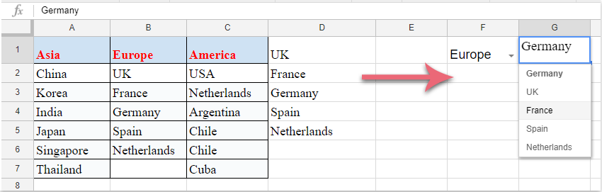
5. Son olarak, Kaydet düğmesine tıklayın ve ikinci bağımlı açılır liste aşağıdaki ekran görüntüsünde gösterildiği gibi başarıyla oluşturulmuştur:
En İyi Ofis Verimlilik Araçları
Kutools for Excel ile Excel becerilerinizi güçlendirin ve benzersiz bir verimlilik deneyimi yaşayın. Kutools for Excel, üretkenliği artırmak ve zamandan tasarruf etmek için300'den fazla Gelişmiş Özellik sunuyor. İhtiyacınız olan özelliği almak için buraya tıklayın...
Office Tab, Ofis uygulamalarına sekmeli arayüz kazandırır ve işinizi çok daha kolaylaştırır.
- Word, Excel, PowerPoint'te sekmeli düzenleme ve okuma işlevini etkinleştirin.
- Yeni pencereler yerine aynı pencerede yeni sekmelerde birden fazla belge açıp oluşturun.
- Verimliliğinizi %50 artırır ve her gün yüzlerce mouse tıklaması azaltır!
Tüm Kutools eklentileri. Tek kurulum
Kutools for Office paketi, Excel, Word, Outlook & PowerPoint için eklentileri ve Office Tab Pro'yu bir araya getirir; Office uygulamalarında çalışan ekipler için ideal bir çözümdür.
- Hepsi bir arada paket — Excel, Word, Outlook & PowerPoint eklentileri + Office Tab Pro
- Tek kurulum, tek lisans — dakikalar içinde kurulun (MSI hazır)
- Birlikte daha verimli — Ofis uygulamalarında hızlı üretkenlik
- 30 günlük tam özellikli deneme — kayıt yok, kredi kartı yok
- En iyi değer — tek tek eklenti almak yerine tasarruf edin