Google Sheets'te başka bir sayfaya dayalı koşullu biçimlendirme nasıl yapılır?
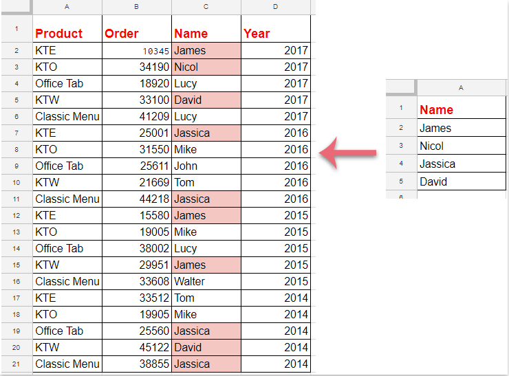
Koşullu biçimlendirme, Google Sheets'te belirli kriterlere göre hücreleri otomatik olarak vurgulamanıza olanak tanıyan kullanışlı bir özelliktir. Bu özellik, verilerinizi analiz etmeyi ve görselleştirmeyi kolaylaştırır. Bazen hücreleri aynı sayfadaki değerlerle değil de farklı bir sayfada depolanan bir referans listesi veya kriterlere göre vurgulamak isteyebilirsiniz. Örneğin, aşağıdaki ekran görüntüsünde gösterildiği gibi, başka bir sayfada tutulan listede de görünen hücreleri vurgulamak isteyebilirsiniz. Bu tür görevler, mevcut satışları ana ürün listesiyle karşılaştırdığınızda veya başka bir veri kaynağına göre yinelenen girişleri kontrol ettiğinizde gibi çapraz referanslı verilerle çalışırken yaygındır. Ancak, özellikle sayfalar arasında veri başvurusu gerektiren durumlarda bu tür koşullu biçimlendirmeyi ayarlamak, daha önce yapmadıysanız kafa karıştırıcı olabilir. Aşağıdaki kılavuz, size adım adım basit bir yöntem gösterecektir.
Google Sheets'te başka bir sayfadan alınan bir listeye dayalı koşullu biçimlendirme
Google Sheets'te başka bir sayfadan alınan bir listeye dayalı koşullu biçimlendirme
Bu yöntem, aktif sayfanızdaki belirli bir listede bulunan hücreleri vurgulamak için bir koşullu format kuralı oluşturmanızı sağlar. Böyle bir çapraz sayfa koşullu biçimlendirme, dinamik veri izleme ve ilişkili veri setleri arasındaki tutarlılığı korumak için özellikle yararlıdır.
Bu süreci tamamlamak için aşağıdaki ayrıntılı adımları izleyin:
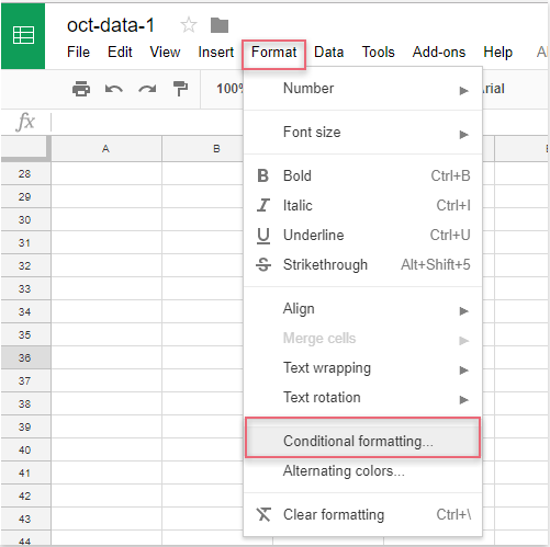
1. Hedef çalışma sayfanızı açın, ardından üstteki Biçim menüsüne tıklayın ve Koşullu biçimlendirme'yi seçin. Koşullu biçim kuralları paneli ekranınızın sağ tarafında açılacaktır.
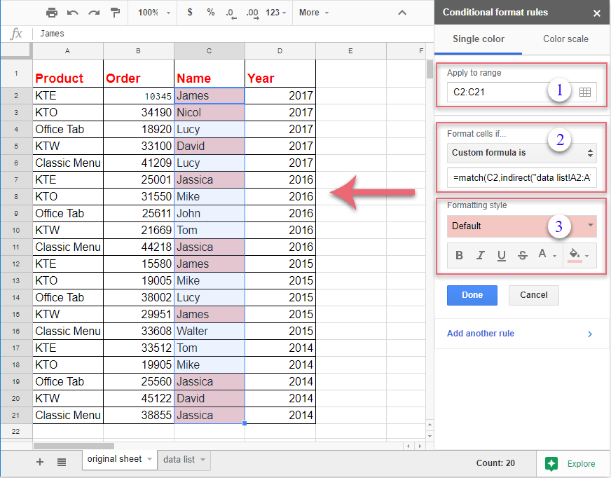
2. Koşullu format kuralları panelinde aşağıdaki işlemleri yapın:
(1.) "Uygula aralığı" alanının yanındaki ![]() düğmesine tıklayın. Vurgulamak istediğiniz hücre aralığını seçin. Örneğin, 2. satırdan itibaren C sütunundaki tüm değerleri biçimlendirmek istiyorsanız, seçin C2:C. Uygun bir aralık seçmek, yalnızca amaçlanan hücrelerin biçimlendirme için değerlendirilmesini sağlar.
düğmesine tıklayın. Vurgulamak istediğiniz hücre aralığını seçin. Örneğin, 2. satırdan itibaren C sütunundaki tüm değerleri biçimlendirmek istiyorsanız, seçin C2:C. Uygun bir aralık seçmek, yalnızca amaçlanan hücrelerin biçimlendirme için değerlendirilmesini sağlar.
(2.) Hücreleri biçimlendir eğer açılır menüsünde Özel formül seçeneğini işaretleyin. Sağlanan kutuya aşağıdaki formülü girin: =match(C2,indirect("data list!A2:A"),0). Bu formül, C sütunundaki her hücrenin "data list" sayfasındaki A2:A aralığındaki herhangi bir değerle eşleşip eşleşmediğini kontrol eder.
(3.) Biçimlendirme stili altında, hücreyi belirli bir renkle doldurma veya yazı tipi stilini değiştirme gibi istenen biçimlendirmeyi seçin. Biçimlendirmeyi uygulamadan önce sayfanızda hemen önizleyebilirsiniz.
Not: Yukarıdaki formülde, C2 seçilen aralıktaki ilk hücreye (verileriniz farklı bir satır veya sütunda başlıyorsa buna göre ayarlayın) ve data list!A2:A ise diğer sayfadan gelen listenizin bulunduğu sayfa adı (“data list”) ve ilgili aralık (A2:A)'ya atıfta bulunur. Formüldeki hücre referansının seçilen aralığınızın sol üst hücresiyle eşleştiğinden emin olun, aksi takdirde biçimlendirme doğru şekilde uygulanmayabilir. Veri listeniz farklı bir aralıksa, formülde buna göre güncelleyin (örneğin, “data list!B2:B”).
3. Kuralı ayarladıktan sonra, seçtiğiniz aralıktaki eşleşen hücreler diğer sayfadan gelen listeye göre anında vurgulanacaktır. Önizlemeyi gözden geçirin, ardından Koşullu format kuralları panelinin altındaki Tamam düğmesine tıklayarak biçimlendirmeyi uygulayıp kaydedin.
İpuçları ve sorun giderme:
- Formülünüzde yazım hatalarını, özellikle sayfa adlarında ve aralık referanslarında iki kez kontrol edin—yanlış referanslar, kuralların uygulanmamasının yaygın nedenlerindendir.
- Veri listeniz boş hücreler içeriyorsa,
MATCHişlevi eşleşmeyen değerler için#YOKhatası döndürür, ancak bu beklenen bir davranıştır ve eşleşen öğelerin vurgulanmasını etkilemez. - Biçimlendirmeyi yeni bir sayfaya kopyaladığınızda veya aralıkları ayarladığınızda, özel formülünüzdaki hücre referanslarını da buna göre güncellediğinizden emin olun.
- Referans listenize daha sonra öğe eklerseniz veya kaldırırsanız, biçimlendirme otomatik olarak güncellenir.
- Formülünüzde belirtilen sayfa ve aralık var ve doğru yazılmış.
- Formülünüzdeki ilk hücre, seçilen aralığınızın ilk hücresiyle eşleşiyor.
- Çalışma sayfanız içinde çapraz sayfa erişimi için gereken tüm izinler mevcut—bu yöntem tek bir çoklu sayfalı Google Sheets dosyası içinde çalışır, farklı dosyalar arasında çalışmaz.
Alternatif olarak, veri yapınız veya gereksinimleriniz daha karmaşıksa—örneğin, birden fazla sütunu karşılaştırmak, kısmi eşleşmelere izin vermek veya daha gelişmiş aramalar yapmak istiyorsanız—COUNTIF veya VLOOKUP formülleri içeren yardımcı sütunlar kullanmak veya Google Apps Script (özel JavaScript kodu) kullanmak da esnek koşullu biçimlendirme çözümleri sağlayabilir.
Özetle, başka bir sayfaya dayalı koşullu biçimlendirme ayarlamak, liste kontrolü, yinelenen izleme ve çeşitli çapraz sayfa veri doğrulamaları için oldukça etkilidir—tüm bunlar Google Sheets içinde gerçekleşir. Sorunsuz ve doğru sonuçlar için formül girişlerinizi, referans aralıklarınızı ve biçimlendirme kurallarınızı her zaman doğrulayın.

Kutools AI ile Excel Sihirini Keşfedin
- Akıllı Yürütme: Hücre işlemleri gerçekleştirin, verileri analiz edin ve grafikler oluşturun—tümü basit komutlarla sürülür.
- Özel Formüller: İş akışlarınızı hızlandırmak için özel formüller oluşturun.
- VBA Kodlama: VBA kodunu kolayca yazın ve uygulayın.
- Formül Yorumlama: Karmaşık formülleri kolayca anlayın.
- Metin Çevirisi: Elektronik tablolarınız içindeki dil engellerini aşın.
En İyi Ofis Verimlilik Araçları
Kutools for Excel ile Excel becerilerinizi güçlendirin ve benzersiz bir verimlilik deneyimi yaşayın. Kutools for Excel, üretkenliği artırmak ve zamandan tasarruf etmek için300'den fazla Gelişmiş Özellik sunuyor. İhtiyacınız olan özelliği almak için buraya tıklayın...
Office Tab, Ofis uygulamalarına sekmeli arayüz kazandırır ve işinizi çok daha kolaylaştırır.
- Word, Excel, PowerPoint'te sekmeli düzenleme ve okuma işlevini etkinleştirin.
- Yeni pencereler yerine aynı pencerede yeni sekmelerde birden fazla belge açıp oluşturun.
- Verimliliğinizi %50 artırır ve her gün yüzlerce mouse tıklaması azaltır!
Tüm Kutools eklentileri. Tek kurulum
Kutools for Office paketi, Excel, Word, Outlook & PowerPoint için eklentileri ve Office Tab Pro'yu bir araya getirir; Office uygulamalarında çalışan ekipler için ideal bir çözümdür.
- Hepsi bir arada paket — Excel, Word, Outlook & PowerPoint eklentileri + Office Tab Pro
- Tek kurulum, tek lisans — dakikalar içinde kurulun (MSI hazır)
- Birlikte daha verimli — Ofis uygulamalarında hızlı üretkenlik
- 30 günlük tam özellikli deneme — kayıt yok, kredi kartı yok
- En iyi değer — tek tek eklenti almak yerine tasarruf edin