Ana içeriğe atla

Excel'de belirli bir aralıkta belirli bir değer varsa bir değer nasıl döndürülür?

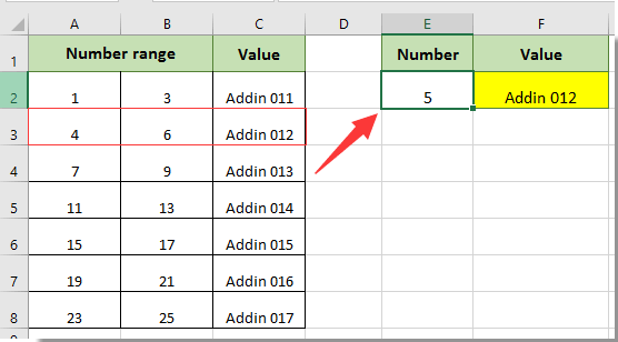
Soldaki ekran görüntüsünde gösterildiği gibi, verilen bir sayı 5 belirli bir sayı aralığındaysa, bitişik hücrede değerin nasıl döndürüleceği. Bu makaledeki formül yöntemi, bunu başarmanıza yardımcı olabilir.

Belirli bir değer belirli bir aralıkta mevcutsa, formül kullanarak bir değer döndür


Belirli bir değer belirli bir aralıkta mevcutsa, formül kullanarak bir değer döndür

Excel'de belirli bir aralıkta belirli bir değer varsa, bir değer döndürmek için lütfen aşağıdaki formülü uygulayın.

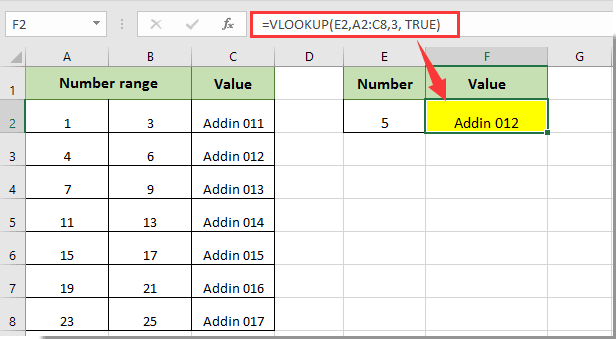
1. Boş bir hücre seçin, formül girin = DÜŞEYARA (E2, A2: C8,3, DOĞRU) Formül Çubuğuna girin ve ardından Keşfet anahtar. Ekran görüntüsüne bakın:

Verilen 5 sayısının 4-6 sayı aralığında olduğunu görebilirsiniz, ardından bitişik hücrede karşılık gelen Addin 012 değeri, yukarıdaki ekran görüntüsünde gösterildiği gibi hemen seçilen hücreye doldurulur.

Notlar: Formülde, E2, hücrenin verilen sayıyı, A2: C8, sayı aralığını ve verilen sayıya göre döndüreceğiniz değeri içerir ve 3 sayısı, döndüreceğiniz değerin üçüncü sütununda yer aldığı anlamına gelir. aralık A2: C8. Lütfen ihtiyacınıza göre değiştirin.


İlgili Makaleler:

En İyi Ofis Üretkenlik Araçları

🤖 Kutools AI Yardımcısı: Aşağıdakilere dayalı olarak veri analizinde devrim yaratın: Akıllı Yürütme   |  Kodunu oluşturun  |  Özel Formüller Oluşturun  |  Verileri Analiz Edin ve Grafikler Oluşturun  |  Kutools İşlevlerini Çağır...
Popüler Özellikler: Yinelenenleri Bul, Vurgula veya Tanımla   |  Boş Satırları Sil   |  Veri Kaybı Olmadan Sütunları veya Hücreleri Birleştirin   |   Formülsüz Tur ...
Süper Arama: Çoklu Ölçütlü VLookup    Çoklu Değer VLookup  |   Birden Çok Sayfada VLookup   |   Bulanık Arama ....
Gelişmiş Açılır Liste: Hızla Açılır Liste Oluşturun   |  Bağımlı Açılır Liste   |  Çoklu Seçim Açılır Liste ....
Sütun Yöneticisi: Belirli Sayıda Sütun Ekleme  |  Sütunları Taşı  |  Gizli Sütunların Görünürlük Durumunu Değiştir  |  Aralıkları ve Sütunları Karşılaştırın ...
Öne Çıkan Özellikler: Izgara Odağı   |  Tasarım görünümü   |   Büyük Formül Çubuğu    Çalışma Kitabı ve Sayfa Yöneticisi   |  Kaynak Kütüphanesi (Otomatik metin)   |  Tarih Seçici   |  Çalışma Sayfalarını Birleştirin   |  Hücreleri Şifrele/Şifresini Çöz    E-postaları Listeye Göre Gönder   |  Süper Filtre   |   Özel Filtre (kalın/italik/üstü çizili filtre...) ...
En İyi 15 Araç Seti12 Metin Tools (Metin ekle, Karakterleri Kaldır, ...)   |   50+ Grafik Türleri (Gantt şeması, ...)   |   40+ Pratik Formüller (Yaşı doğum gününe göre hesapla, ...)   |   19 sokma Tools (QR Kodunu Girin, Yoldan Resim Ekle, ...)   |   12 Dönüştürme Tools (Sayılardan Kelimelere, Para Birimi Dönüştürme, ...)   |   7 Birleştir ve Böl Tools (Gelişmiş Kombine Satırları, Bölünmüş hücreler, ...)   |   ... ve dahası

Kutools for Excel ile Excel Becerilerinizi Güçlendirin ve Daha Önce Hiç Olmadığı Gibi Verimliliği Deneyimleyin. Kutools for Excel, Üretkenliği Artırmak ve Zamandan Tasarruf Etmek için 300'den Fazla Gelişmiş Özellik Sunar.  En Çok İhtiyacınız Olan Özelliği Almak İçin Buraya Tıklayın...

Açıklama


Office Tab, Office'e Sekmeli Arayüz Getirir ve İşinizi Çok Daha Kolay Hale Getirir

  • Word, Excel, PowerPoint'te sekmeli düzenlemeyi ve okumayı etkinleştirin, Publisher, Access, Visio ve Project.
  • Yeni pencereler yerine aynı pencerenin yeni sekmelerinde birden çok belge açın ve oluşturun.
  • Üretkenliğinizi% 50 artırır ve her gün sizin için yüzlerce fare tıklamasını azaltır!
Comments (14)
No ratings yet. Be the first to rate!
This comment was minimized by the moderator on the site
Prezados,
Bom dia!

É possível determinar algum parâmetro dentro do Range.

Quero fazer o PROCV trazer de um intervalo, porém ele acaba retornando valores de CEPs que não existem, mas que estão muito próximos...

Exemplo:

Na tabela existe a faixa de CEP 68795000 A 68796999 que é do estado do Pará
Ao utilizar as formula sugeridas, resulta como "verdadeiro" para a faixa de CEP 69301000 A 69390971 que é do estado de Roraima, devido a proximidade da numeração.
This comment was minimized by the moderator on the site
Hi Nilton Vanini,
I don't quite understand your question. Do you mind uploading a screenshot of your data? Sorry for the inconvenience.
This comment was minimized by the moderator on the site
This seems to also work with text. I got this to work with exact value rather than a range by using the "Value" column as part of the range in the formula.

My question is, are you forced to use 2 columns or is it possible to only use 1 and the value column?

I created a master sheet to call from but this is how I setup the formla

=VLOOKUP(I2,'Master Sheet'!$A$2:$B$53,2,TRUE)

Column "I" text (Number column in the example), I was forced to have a range so column "B" is both the Range and Value.

Is this best practice or would I run into unexpected issues down the road if more line items are added to this list?
This comment was minimized by the moderator on the site
Hi Andrew,
You may need to upload a screenshot of your data. Sorry for the inconvenience.
This comment was minimized by the moderator on the site
Bonjour je cherche à vérifier si une de mes valeurs correspond à une plage de données, le problème est que je n'ai pas qu'une valeur à vérifier mais une longue liste. J'aimerais que si une des 3 valeurs suivantes que je tape dans une case (exemple "panneau";"Strat";"chants") correspondent à une plage de données, elles 's'affichent en rouge par exemple. Sauriez vous me renseigner ? Merci.
This comment was minimized by the moderator on the site
Yo quiero devolver 1, si se encuentra en un rango de numeros determinados, ej. el rango es de 4 a 10, y en la celda tengo 5, devolver 1, pero si tengo 2 o 15, devolver 0.
This comment was minimized by the moderator on the site
Hi Daili,
If you just want to check if a number exists in a given range and return a specified value, you can combine IF with AND functions to get it done.
Suppose the number 4 is in cell A9, the number 10 is in cell B9, the number you want to determine if it exists between 4 and 10 is locateed in D9, you can apply the following formula to get the correct result.
=IF(AND(D9>A9,D9<B9),1,0)
This comment was minimized by the moderator on the site
Can you do a lookup searching a range of 3digit zips (i.e. 010-013 or 280-283,286,297) and pull in the city / state from your zip code list. The zip code list is all 3 digit zips in US broken out individually. The zips are listed multiple times because there are several city / state combinations. (i.e. 010 Ludlow MA; 010 Plamer MA etc).
This comment was minimized by the moderator on the site
The value works on the first cell. How do you do it for the entire column cell?
This comment was minimized by the moderator on the site
You will need to use $ for the lookup cells values
So if you have a column of values you want to look up you would modify the formula as follows:
=VLOOKUP(E2,$A$2:$C$8,3, TRUE)

E2 would change as you fill down but the table you are looking up from will remain constant
This comment was minimized by the moderator on the site
awesome, thanks!
This comment was minimized by the moderator on the site
Doesn't work. if only it was that simple, wouldn't need to be googling for this
This comment was minimized by the moderator on the site
It obviously does. Instead of whining and trying to be a smartass about it, you could have at least tried it out.
This comment was minimized by the moderator on the site
It does. Try it out before rudely complaining, simple as that.
There are no comments posted here yet
Please leave your comments in English
Posting as Guest
×
Rate this post:
0   Characters
Suggested Locations