Excel tablosundan birden fazla sütun döndürmek için vlookup nasıl kullanılır?
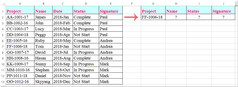
Excel çalışma sayfasında, bir sütundan eşleşen değeri döndürmek için Vlookup işlevini kullanabilirsiniz. Ancak, bazen aşağıdaki ekran görüntüsünde gösterildiği gibi, birden fazla sütundan eşleşen değerleri çıkarmak isteyebilirsiniz. Vlookup işlevini kullanarak aynı anda birden fazla sütundan karşılık gelen değerleri nasıl alabilirsiniz?
Dizi formülü ile birden fazla sütundan Vlookup eşleşen değerler
Dizi formülü ile birden fazla sütundan Vlookup eşleşen değerler
Burada, size birden fazla sütundan eşleşen değerleri döndürmek için Vlookup işlevini tanıtacağım, lütfen şu adımları izleyin:
1. Birden fazla sütundan eşleşen değerleri yerleştirmek istediğiniz hücreleri seçin, aşağıdaki ekran görüntüsüne bakın:

2. Ardından aşağıdaki formülü formül çubuğuna girin ve sonra Ctrl + Shift + Enter tuşlarına birlikte basın, ve birden fazla sütundan eşleşen değerler anında çıkarılmış olacaktır, aşağıdaki ekran görüntüsüne bakın:
=VLOOKUP(G2,A1:E13,{2,4,5},FALSE)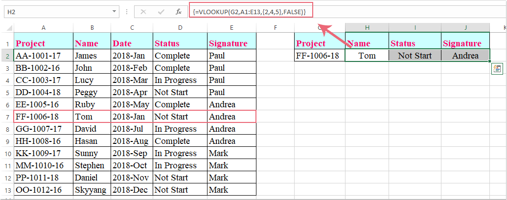
Not: Yukarıdaki formülde, G2 döndürülecek değerlere dayanmak istediğiniz kriterdir, A1:E13 vlookup yapmak istediğiniz tablo aralığıdır, 2, 4, 5 sayıları ise değerleri döndürmek istediğiniz sütun numaralarıdır.
Kutools ile VLOOKUP Sınırlarını Aşın: Süper ARA
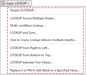
Excel'deki VLOOKUP fonksiyonunun sınırlamalarını gidermek için Kutools, kullanıcılara daha güçlü ve esnek bir veri arama çözümü sunan birden fazla gelişmiş ARA özelliği geliştirmiştir.
- 🔍 Çoklu sayfa araması...: Eşleşen verileri bulmak için birden fazla çalışma sayfasında arama yapın.
- 📝 Çoklu Koşul Araması...: Aynı anda birden fazla kriteri karşılayan verileri arayın.
- ➕ Ara ve Topla...: Bir arama değerine göre verileri arayın ve sonuçları toplayın.
- 📋 Birçoklu arama (birden fazla sonuç döndürme)...: Tek bir arama girdisi için birden fazla eşleşen değeri alın.
- Kutools For Excel'i Şimdi Edinin!
En İyi Ofis Verimlilik Araçları
Kutools for Excel ile Excel becerilerinizi güçlendirin ve benzersiz bir verimlilik deneyimi yaşayın. Kutools for Excel, üretkenliği artırmak ve zamandan tasarruf etmek için300'den fazla Gelişmiş Özellik sunuyor. İhtiyacınız olan özelliği almak için buraya tıklayın...
Office Tab, Ofis uygulamalarına sekmeli arayüz kazandırır ve işinizi çok daha kolaylaştırır.
- Word, Excel, PowerPoint'te sekmeli düzenleme ve okuma işlevini etkinleştirin.
- Yeni pencereler yerine aynı pencerede yeni sekmelerde birden fazla belge açıp oluşturun.
- Verimliliğinizi %50 artırır ve her gün yüzlerce mouse tıklaması azaltır!
Tüm Kutools eklentileri. Tek kurulum
Kutools for Office paketi, Excel, Word, Outlook & PowerPoint için eklentileri ve Office Tab Pro'yu bir araya getirir; Office uygulamalarında çalışan ekipler için ideal bir çözümdür.
- Hepsi bir arada paket — Excel, Word, Outlook & PowerPoint eklentileri + Office Tab Pro
- Tek kurulum, tek lisans — dakikalar içinde kurulun (MSI hazır)
- Birlikte daha verimli — Ofis uygulamalarında hızlı üretkenlik
- 30 günlük tam özellikli deneme — kayıt yok, kredi kartı yok
- En iyi değer — tek tek eklenti almak yerine tasarruf edin