Ana içeriğe atla

Excel'de bir veya birden çok ölçüt temelinde birden çok eşleşen değer nasıl döndürülür?

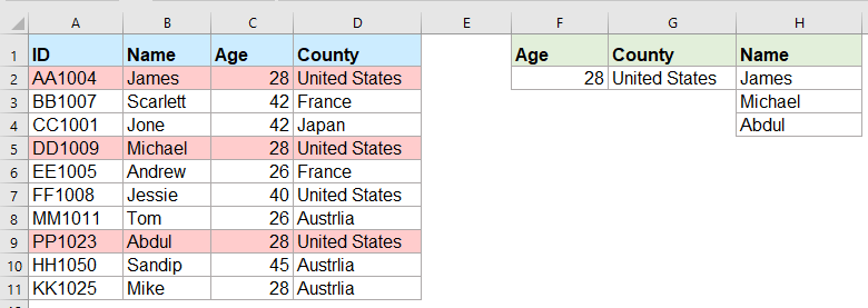
Normalde, belirli bir değeri aramak ve eşleşen öğeyi döndürmek, DÜŞEYARA işlevini kullanarak çoğumuz için kolaydır. Ancak, aşağıda gösterilen ekran görüntüsü gibi bir veya daha fazla kritere göre birden çok eşleşen değer döndürmeyi denediniz mi? Bu yazıda, bu karmaşık görevi Excel'de çözmek için bazı formüller tanıtacağım.

Dizi formülleriyle bir veya birden çok ölçüte göre birden çok eşleşen değer döndür


Dizi formülleriyle bir veya birden çok ölçüte göre birden çok eşleşen değer döndür

Örneğin, yaşı 28 olan ve Amerika Birleşik Devletleri'nden gelen tüm isimleri çıkarmak istiyorum, lütfen aşağıdaki formülü uygulayın:

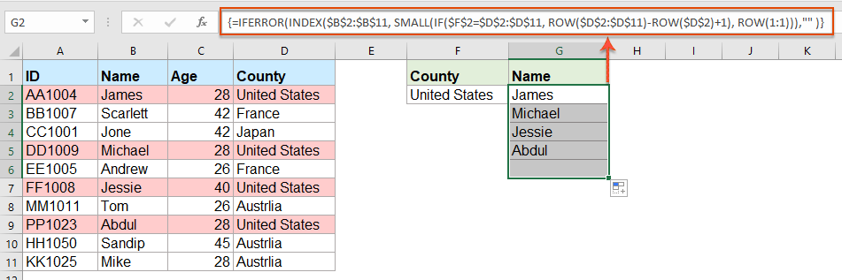
1. Aşağıdaki formülü kopyalayın veya sonucu bulmak istediğiniz boş bir hücreye girin:

=INDEX($B$2:$B$11, SMALL(IF(COUNTIF($F$2, $C$2:$C$11)*COUNTIF($G$2, $D$2:$D$11), ROW($A$2:$D$11)-MIN(ROW($A$2:$D$11))+1), ROW(A1)), COLUMN(A1))

not: Yukarıdaki formülde, B2: B11 eşleşen değerin döndürüldüğü sütundur; F2, C2: C11 ilk koşul ve ilk koşulu içeren sütun verileridir; G2, D2: D11 ikinci koşul ve bu durumu içeren sütun verileridir, lütfen bunları ihtiyacınıza göre değiştirin.

2. Daha sonra, tuşuna basın. Ctrl + Üst Karakter + Enter ilk eşleşen sonucu almak için tuşlarını kullanın ve ardından ilk formül hücresini seçin ve doldurma tutamacını hata değeri görüntülenene kadar hücrelere sürükleyin, şimdi tüm eşleşen değerler aşağıda gösterilen ekran görüntüsü gibi döndürülür:

İpuçları: Tüm eşleşen değerleri tek bir koşula göre döndürmeniz gerekiyorsa, lütfen aşağıdaki dizi formülünü uygulayın:

=IFERROR(INDEX($B$2:$B$11, SMALL(IF($F$2=$D$2:$D$11, ROW($D$2:$D$11)-ROW($D$2)+1), ROW(1:1))),"" )


Daha ilgili makaleler:

  • Virgülle Ayrılmış Bir Hücrede Birden Çok Arama Değerini Döndür
  • Excel'de, bir tablo hücresinden ilk eşleşen değeri döndürmek için DÜŞEYARA işlevini uygulayabiliriz, ancak bazen, tüm eşleşen değerleri ayıklamamız ve ardından virgül, tire, vb. Gibi belirli bir sınırlayıcıyla tek bir Aşağıdaki ekran görüntüsü gibi hücre. Excel'de virgülle ayrılmış tek bir hücrede birden çok arama değerini nasıl alabilir ve döndürebiliriz?
  • Vlookup Ve Google E-Tablosunda Aynı Anda Birden Çok Eşleşen Değer Döndür
  • Google sayfasındaki normal Vlookup işlevi, belirli bir veriye dayalı olarak ilk eşleşen değeri bulmanıza ve döndürmenize yardımcı olabilir. Ancak bazen, aşağıdaki ekran görüntüsü gibi tüm eşleşen değerleri görüntülemeniz ve döndürmeniz gerekebilir. Bu görevi Google sayfasında çözmenin iyi ve kolay yolları var mı?
  • Vlookup ve Açılır Listeden Birden Çok Değer Döndür
  • Excel'de, bir açılır listeden birden fazla karşılık gelen değeri nasıl görüntüleyebilir ve döndürebilirsiniz; bu, açılır listeden bir öğe seçtiğinizde, aşağıdaki ekran görüntüsü gibi tüm göreli değerleri aynı anda görüntülenir. Bu yazıda çözümü adım adım tanıtacağım.
  • Vlookup ve Excel'de Çoklu Değerleri Dikey Olarak Döndür
  • Normalde, ilk karşılık gelen değeri almak için Vlookup işlevini kullanabilirsiniz, ancak bazen, eşleşen tüm kayıtları belirli bir kritere göre döndürmek istersiniz. Bu yazıda, tüm eşleşen değerlerin dikey, yatay veya tek bir hücreye nasıl bakılacağı ve döndürüleceği hakkında konuşacağım.
  • Excel'de İki Değer Arasında Vlookup ve Dönüş Eşleştirme Verileri
  • Excel'de, belirli bir veriye dayalı olarak karşılık gelen değeri elde etmek için normal Vlookup işlevini uygulayabiliriz. Ancak, bazen, aşağıdaki ekran görüntüsünde gösterildiği gibi, iki değer arasındaki eşleşen değeri vlookup ve döndürmek istiyoruz, bu görevi Excel'de nasıl halledebilirsiniz?


  • Süper Formül Çubuğu (birden çok metin ve formül satırını kolayca düzenleyin); Okuma Düzeni (çok sayıda hücreyi kolayca okuyun ve düzenleyin); Filtrelenmiş Aralığa Yapıştır...
  • Hücreleri / Satırları / Sütunları Birleştirme ve Verilerin Saklanması; Bölünmüş Hücre İçeriği; Yinelenen Satırları ve Toplam / Ortalamayı Birleştirme... Yinelenen Hücreleri Önleyin; Aralıkları Karşılaştır...
  • Yinelenen veya Benzersiz'i seçin Satırlar; Boş Satırları Seçin (tüm hücreler boştur); Süper Bul ve Bulanık Bul Birçok Çalışma Kitabında; Rastgele Seçim ...
  • Tam kopya Formül referansını değiştirmeden Birden Çok Hücre; Otomatik Referans Oluştur Birden Çok Sayfaya; Madde İşaretleri Ekle, Onay Kutuları ve daha fazlası ...
  • Sık Kullanılan ve Hızlı Eklenen Formüller, Aralıklar, Grafikler ve Resimler; Hücreleri Şifrele şifre ile; Posta Listesi Oluşturun ve e-posta gönder ...
  • Metni Çıkar, Metin Ekle, Konuma Göre Kaldır, Alanı Kaldır; Sayfalama Alt Toplamları Oluşturma ve Yazdırma; Hücre İçeriği ve Yorumları Arasında Dönüştür...
  • Süper Filtre (filtre şemalarını kaydedin ve diğer sayfalara uygulayın); Gelişmiş Sıralama ay / hafta / gün, sıklık ve daha fazlasına göre; Özel Filtre kalın, italik ...
  • Çalışma Kitaplarını ve Çalışma Sayfalarını Birleştirin; Tabloları anahtar sütunlara göre birleştirin; Verileri Birden Çok Sayfaya Bölme; Toplu dönüştürme xls, xlsx ve PDF...
  • Pivot Tablo Gruplaması hafta numarası, haftanın günü ve daha fazlası ... Kilidi Açılmış, Kilitli Hücreleri Göster farklı renklerle; Formülü / Adı Olan Hücreleri Vurgulayın...
kte sekmesi 201905
  • Word, Excel, PowerPoint'te sekmeli düzenlemeyi ve okumayı etkinleştirin, Publisher, Access, Visio ve Project.
  • Yeni pencereler yerine aynı pencerenin yeni sekmelerinde birden çok belge açın ve oluşturun.
  • Üretkenliğinizi% 50 artırır ve her gün sizin için yüzlerce fare tıklamasını azaltır!
ofis tabanı


Comments (25)
No ratings yet. Be the first to rate!
This comment was minimized by the moderator on the site
Hi, if there are duplicate values (e.g. two adams), how do i make sure that it only returns 1 adam and not 2?
This comment was minimized by the moderator on the site
Hello, Bobby,
To extract only unique matching values, you should apply the below formula:
After pasting the formula, please press Ctrl + Shift + Enter keys together to get the correct result.
=IFERROR(INDEX($B$2:$B$5, MATCH(0, COUNTIF(H1:$H$1, $B$2:$B$5)+IF($D$2:$D$5<>$G$2, 1, 0)+IF($C$2:$C$5<>$F$2, 1, 0), 0)), "")

Please have a try, hope it can help you!
This comment was minimized by the moderator on the site
Hi,

Thanks for posting these examples.
I'm trying to implement this in my own sheet, but don't get it to work (maybe because I'm using an europe version of excel)?

I want to get the dates of the days that I had my shifts or that I have worked 'some' (>0) hours for a client.

So in I3 is the name and in J3 the month. K3 and L3 are the shifts (1 is worked) and hours (don't know how to set this, should be more than zero)

My expected results are in:
Shifts: I7 and I8
hours: J7

So I worked more than 0 hours for 'person 2' in oktober on 3-10-2022
had shifts for person 2 on '10-10-2022' and 28-10-2022

When I add '=INDEX($B$2:$B$11, SMALL(IF(COUNTIF($F$2, $C$2:$C$11)*COUNTIF($G$2, $D$2:$D$11), ROW($A$2:$D$11)-MIN(ROW($A$2:$D$11))+1), ROW(A1)), COLUMN(A1))' in my excel sheet, it doesn't allow the comma between the different parts of the formula.
So I need to change them to ';'.
But when I try it it always says: '#NAME?'

So can someone help me with this?

Kind regards,

Bas
[img]https://drive.google.com/file/d/1iIPQKuj_PNhqWyWlwJ4IQTqGNEd6B9Hw/view?usp=share_link[/img]
This comment was minimized by the moderator on the site
Hi,

First, thank you for sharing!

Can you please provide a solution to the case below:

I have 3 columns (A: Containing reference information, B: Containing information to be searched, C: Search result)

Image url is provided below

https://ibb.co/VHCd09K

Column A-------------------------Column B------------Column C
File Name-------------------------Name----------------File Name, Document Name, Element Name, Name
Changed Element-----------------Element--------------Changed Element, Element Name, Element ID
Column Location
Document Name
Element Name
Name
Category
Warranty
Slope
Element ID

What I need is to search in column A for any partial match with cell B2 (Name) or B3 (Element) and get the result in one cell,

Thank you, Behzad
This comment was minimized by the moderator on the site
Hello, Behzad
Maybe the below User Defined Function can help you.
Public Function ConcatPartLookUp(rngInput As Range, rngSource As Range, Optional strDelimiter As String, Optional blCaseSensitive)
Dim rng As Range
If strDelimiter = "" Then strDelimiter = ","
If IsMissing(blCaseSensitive) Then
    blCaseSensitive = False
Else
    blCaseSensitive = True
End If
For Each rng In rngSource
    If blCaseSensitive Then
        If InStr(1, rng.Value, rngInput.Value, vbBinaryCompare) > 0 Then ConcatPartLookUp = ConcatPartLookUp & strDelimiter & rng.Value
    Else
        If InStr(1, rng.Value, rngInput.Value, vbTextCompare) > 0 Then ConcatPartLookUp = ConcatPartLookUp & strDelimiter & rng.Value
    End If
Next
If Len(ConcatPartLookUp) > 0 Then ConcatPartLookUp = Mid(ConcatPartLookUp, 2, Len(ConcatPartLookUp))
End Function


After copying and pasting this code, and then use this formula:=ConcatPartLookUp(B2,$A$2:$A$8) to get the result you need.
Please have a try, hope it can help you!
This comment was minimized by the moderator on the site
Heyi, thank you for the formula. It worked for "fixed" values / text as criterias. However, one of the criterias i'm trying to use is a condition (values <>0 ), but does not work the described formula. Do you guys know what should i change to adapt the formula so I can have a condition as one of the criterias, please?

Best,

João
This comment was minimized by the moderator on the site
Hello, Marcus
To solve your problem, please view this article:
https://www.extendoffice.com/documents/excel/6393-excel-vlookup-function.html#b3-2
There are some detailed explanations of this task. You just need to change the criteira to your own.
Thank you!
This comment was minimized by the moderator on the site
Hi,

if in cell H1 i write "Name" and wanted to link that with the formula, how would that work?
Then I could write "ID" in cell H1 and would automatically get as a result: AA1004; DD1009; PP1023 (for the first formula)

Thank you in advance!
This comment was minimized by the moderator on the site
Hello, Marie
Sorry, i can't get the point of your first problem, could you explain your problem more clearly and detailedly? Or you can insert a screenshot here to describe your problem.
As for the second question, you just need to change the cell reference as this:
=INDEX($A$2:$A$11, SMALL(IF(COUNTIF($F$2, $C$2:$C$11)*COUNTIF($G$2, $D$2:$D$11), ROW($A$2:$D$11)-MIN(ROW($A$2:$D$11))+1), ROW(A1)), COLUMN(A1))

Remeber to press Ctrl + Shift + Enter keys together.
Please try, hope it can help you!
This comment was minimized by the moderator on the site
Hello,
what would be needed to expand the first formula in the following case:
Some IDs are Blank (e.g. cell A5 is blank) and I would like an additional condition outputting lines only when the IDs are not blank. (So the output should then be James and Abdul.
Thanks!
This comment was minimized by the moderator on the site
Hello, Jo,
To solve your problem, please apply the below formula:
=INDEX($B$2:$B$11, SMALL(IF(COUNTIF($F$2, $C$2:$C$11)*COUNTIF($G$2, $D$2:$D$11)*($A$2:$A$11<>0), ROW($A$2:$D$11)-MIN(ROW($A$2:$D$11))+1), ROW(A1)), COLUMN(A1))

Please have a ry, hope it can help you!
This comment was minimized by the moderator on the site
hello,
ive tried using the formula and it either generates a value of 0 or the image attached
This comment was minimized by the moderator on the site
Hello, Milku
Your screenshot showed WPS software of MAC version, so I am not sure whether our formula is available.
I uploaded an Excel file to here, you can try to see if it can calculate correctly in you environment.
Thank you!
This comment was minimized by the moderator on the site
When I use the second formula and drag down, nothing appears. The formula result (fx) says it should be returning something but it is blank. How do I correct this?
This comment was minimized by the moderator on the site
Hello Alysia,

Glad to help. I tried the second formula in the article and drag the formula down, the rest of results were returned. I think there may be two reasons for your problem. First, maybe you forget to press Ctrl + Shift + Enter keys to enter the formula. Second, the matching result is only one, so no other results are not returned. Please have a check.

Sincerely,
Mandy
This comment was minimized by the moderator on the site
Hi,

I was wondering if it at all possible to enter a 2nd criteria but from the same range as the 1st criteria,

For example with the used example above i would like to search for the names of people from both America and France So cell F3 would have France, Scarlett & Andrew would also populate in the list in Column G

Thank you for assistance in advance.
This comment was minimized by the moderator on the site
Hello Nick,

Glad to help. If you want to get the names of people from both America and France, I advise you to use our formula twice to get the result. Please see the screenshot, In F2 and G2 are values "United States" and "France". Apply formula =IFERROR(INDEX($B$2:$B$11, SMALL(IF($F$2=$D$2:$D$11, ROW($D$2:$D$11)-ROW($D$2)+1), ROW(1:1))),"" ) to get the results for America. And apply formula =IFERROR(INDEX($B$2:$B$11, SMALL(IF($G$2=$D$2:$D$11, ROW($D$2:$D$11)-ROW($D$2)+1), ROW(1:1))),"" ) to get the results for France. It's simple. Please have a try.

Sincerely,
Mandy
This comment was minimized by the moderator on the site
In the first example, what change to the formula would be needed to return everyone who was less than 28 years old?
There are no comments posted here yet
Load More
Please leave your comments in English
Posting as Guest
×
Rate this post:
0   Characters
Suggested Locations