Excel'de negatif sayıları pozitife nasıl çevirirsiniz?
Excel'de işlemler gerçekleştirirken, bazen negatif sayıları pozitif sayılara veya tam tersine çevirmeniz gerekebilir. Negatif sayıları pozitife çevirmek için kullanabileceğiniz hızlı yöntemler var mı? Bu makalede, tüm negatif sayıları kolayca pozitif veya tam tersine çevirmek için size aşağıdaki yöntemleri tanıtacağım.
Özel Yapıştır işleviyle negatif sayıları pozitife çevirme
Kutools for Excel ile negatif sayıları kolayca pozitife çevirme
Bir aralıktaki tüm negatif sayıları pozitife çevirmek için VBA kodu kullanma
Özel Yapıştır işleviyle negatif sayıları pozitife çevirme
Negatif sayıları pozitif sayılara aşağıdaki adımları izleyerek değiştirebilirsiniz:
1. Boş bir hücreye -1 sayısını girin, ardından bu hücreyi seçin ve kopyalamak için Ctrl + C tuşlarına basın.
2Aralıktaki tüm negatif sayıları seçin, sağ tıklayın ve Özel Yapıştır... bağlam menüsünden seçin. Ekran görüntüsüne bakın: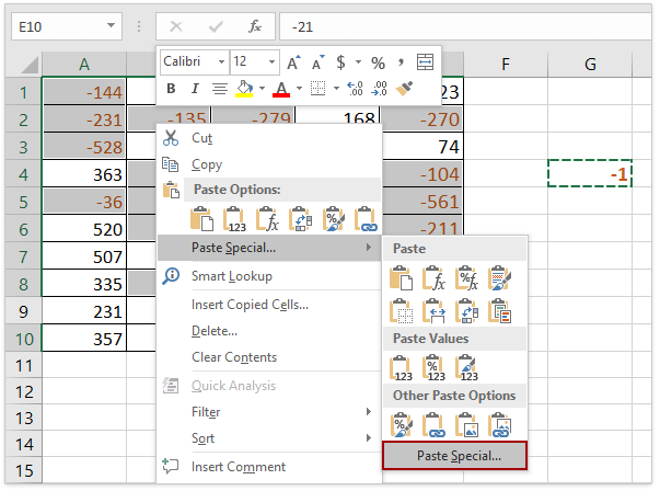
(1) Tuşuna basılı tutarak Ctrl tüm negatif sayıları tek tek tıklayarak seçebilirsiniz;
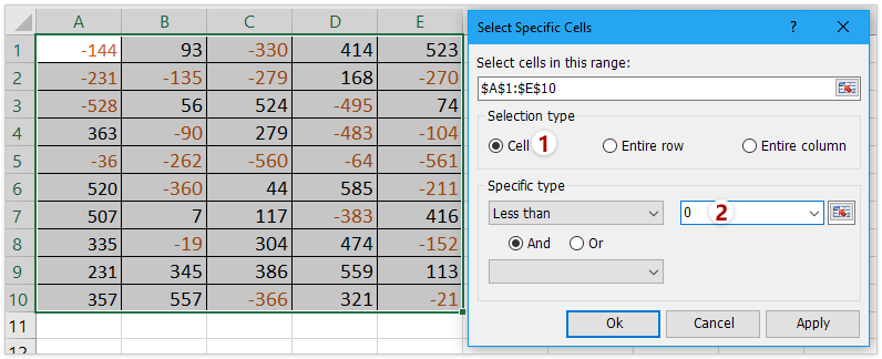
(2) Eğer Kutools for Excel yüklüyse, Özel Hücreleri Seç özelliğini kullanarak tüm negatif sayıları hızlıca seçebilirsiniz. Ücretsiz Deneme Yapın!
3ve bir Özel Yapıştır diyalog kutusu açılacak, Tümünü seçeneğini Yapıştır, select Çarp seçeneğini Hesaplamabölümünden seçin, ardından Tamam'a tıklayın. Ekran görüntüsüne bakın:
4Seçilen tüm negatif sayılar pozitif sayılara dönüştürülecek. İhtiyaç duyduğunuzda -1 sayısını silebilirsiniz. Ekran görüntüsüne bakın:
Kutools for Excel ile negatif sayıları hızlı ve kolay bir şekilde pozitife çevirme
Çoğu Excel kullanıcısı VBA kodunu kullanmak istemiyor, negatif sayıları pozitife çevirmek için hızlı yöntemler var mı? Kutools for Excel, bu işlemi size kolayca ve rahatça gerçekleştirmenize yardımcı olabilir.
1Değiştirmek istediğiniz negatif sayıları içeren bir aralık seçin ve Kutools > Metin > Sayıların işaretini değiştir.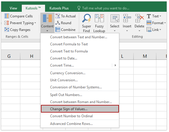
2seçeneğini işaretleyin. Tüm negatif sayıları pozitife çevir seçeneğini Hesaplamabölümünden seçin ve Tamam'a tıklayın. Ekran görüntüsüne bakın: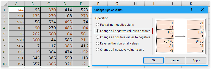
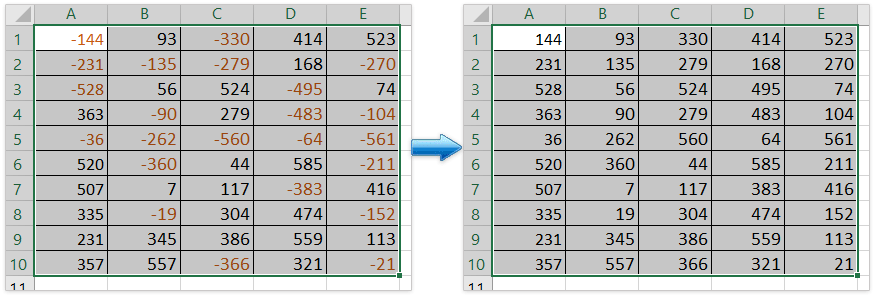
Şimdi tüm negatif sayıların pozitif sayılara dönüştüğünü göreceksiniz, aşağıda gösterildiği gibi: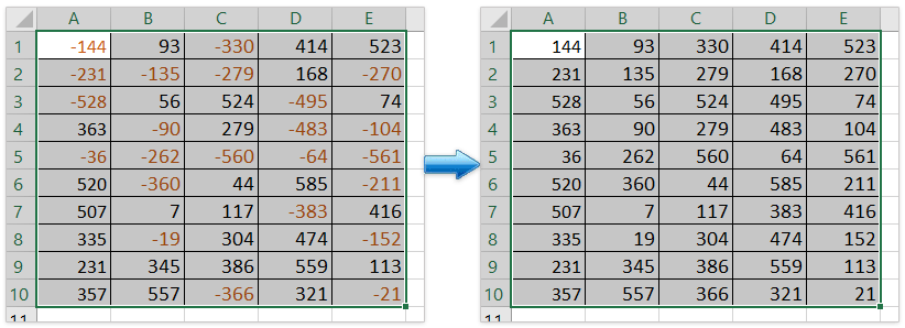
Not: Bu Sayıların İşaretini Değiştir özelliği ile ayrıca sondaki negatif işaretleri düzeltebilir, tüm pozitif sayıları negatife çevirebilir, tüm değerlerin işaretini tersine çevirebilir ve tüm negatif değerleri sıfıra çevirebilirsiniz. Ücretsiz Deneme Yapın!
(1) Belirtilen aralıktaki tüm pozitif değerleri hızlıca negatife çevirme: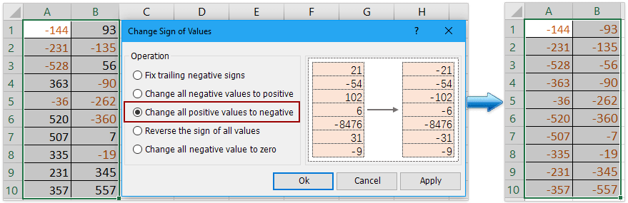
(2) Belirtilen aralıktaki tüm değerlerin işaretini kolayca tersine çevirme: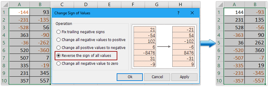
(3) Belirtilen aralıktaki tüm negatif değerleri kolayca sıfıra çevirme:
(4) Belirtilen aralıktaki sondaki negatif işaretleri kolayca düzeltme: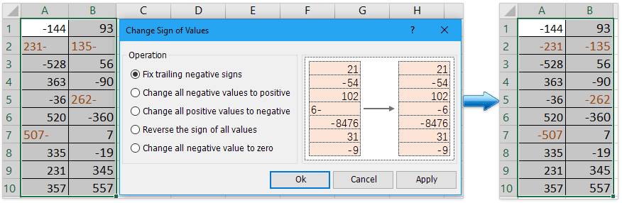
Belirli bir aralıktaki tüm negatif sayıları pozitife çevirmek için VBA kodu kullanma
Excel uzmanı olarak, negatif sayıları pozitif sayılara çevirmek için VBA kodunu da çalıştırabilirsiniz.
1. Microsoft Visual Basic for Applications penceresini açmak için Alt + F11 tuşlarına basın.
2. Yeni bir pencere açılacak. Ekle > Modül'e tıklayın ve ardından aşağıdaki kodları modüle girin:
Sub Positive
Dim Cel As Range
For Each Cel In Selection
If IsNumeric(Cel.Value) Then
Cel.Value = Abs(Cel.Value)
End If
Next Cel
End Sub3Ardından Çalıştır düğmesine tıklayın veya F5 tuşuna basarak uygulamayı çalıştırın ve tüm negatif sayılar pozitif sayılara dönüşecektir. Ekran görüntüsüne bakın:
İlgili makaleler
Hücrelerdeki değerlerin işaretlerini tersine çevirme
Excel'i kullandığımızda, bir çalışma sayfasında hem pozitif hem de negatif sayılar bulunur. Pozitif sayıları negatif ve tam tersine çevirmemiz gerektiğini varsayalım. Elbette bunları manuel olarak değiştirebiliriz, ancak yüzlerce sayı değiştirilmesi gerekiyorsa bu yöntem iyi bir seçenek değildir. Bu sorunu çözmek için hızlı yöntemler var mı?
Pozitif sayıları negatife çevirme
Excel'de tüm pozitif sayıları veya değerleri hızlıca negatife nasıl çevirebilirsiniz? Aşağıdaki yöntemler, Excel'de tüm pozitif sayıları hızlıca negatife çevirmenize rehberlik edecektir.
Hücrelerde sondaki negatif işaretleri düzeltme
Bazı nedenlerden dolayı, Excel'deki hücrelerde sondaki negatif işaretleri düzeltmeniz gerekebilir. Örneğin, sondaki negatif işareti olan bir sayı 90- gibi görünebilir. Bu durumda, sondaki negatif işaretini sağdan sola doğru kaldırarak hızlıca nasıl düzeltebilirsiniz? İşte size yardımcı olabilecek bazı hızlı ipuçları.
Negatif sayıyı sıfıra çevirme
Seçimdeki tüm negatif sayıları aynı anda sıfırlara nasıl çevireceğinizi göstereceğim.
En İyi Ofis Verimlilik Araçları
Kutools for Excel - Kalabalıktan Farklılaşmanızı Sağlar
Kutools for Excel, İhtiyacınız Olan Her Şeyin Bir Tıklama Uzağında Olduğundan Emin Olmak İçin 300'den Fazla Özelliğe Sahiptir...
Office Tab - Microsoft Office'de (Excel Dahil) Sekmeli Okuma ve Düzenlemeyi Etkinleştirin
- Onlarca açık belge arasında bir saniyede geçiş yapın!
- Her gün yüzlerce fare tıklamasından sizi kurtarır, fare eline veda edin.
- Birden fazla belgeyi görüntülediğinizde ve düzenlediğinizde üretkenliğinizi %50 artırır.
- Chrome, Edge ve Firefox gibi Office'e (Excel dahil) Etkin Sekmeler Getirir.