Excel'de hücre değerine göre arka plan veya yazı tipi rengini nasıl değiştirirsiniz?
Excel'de büyük miktarda veriyle uğraşırken, belirli değerleri seçmek ve bunları belirli bir arka plan veya yazı tipi rengiyle vurgulamak isteyebilirsiniz. Bu makale, Excel'de hücre değerlerine göre arka plan veya yazı tipi rengini hızlı bir şekilde değiştirmenin nasıl yapılacağını anlatmaktadır.
Yöntem 1: Koşullu Biçimlendirme ile hücre değerine göre arka plan veya yazı tipi rengini dinamik olarak değiştirme
Koşullu Biçimlendirme özelliği, x'ten büyük, y'den küçük veya x ve y arasında olan değerleri vurgulamanıza yardımcı olabilir.
Diyelim ki elinizde bir dizi veri var ve şimdi 80 ile 100 arasındaki değerleri renklendirmeniz gerekiyor, lütfen aşağıdaki adımları izleyin:
1. Vurgulamak istediğiniz hücre aralığını seçin ve ardından Giriş > Koşullu Biçimlendirme > Yeni Kural'a tıklayın, ekran görüntüsüne bakın:

2. Yeni Biçimlendirme Kuralı iletişim kutusunda, Kural Türü Seç bölümünde yalnızca belirli içerikleri içeren hücreleri biçimlendir seçeneğini belirleyin ve yalnızca şu hücreleri biçimlendir bölümünde gerekli koşulları belirtin:
- İlk açılır kutuda, Hücre Değeri'ni seçin;
- İkinci açılır kutuda, kriter olarak arasında'yı seçin;
- Üçüncü ve dördüncü kutuya, örneğin 80, 100 gibi filtreleme koşullarını girin.

3. Ardından, Biçimlendir düğmesine tıklayın, Hücreleri Biçimlendir iletişim kutusunda, arka plan veya yazı tipi rengini şu şekilde ayarlayın:
| Hücre değerine göre arka plan rengini değiştirme: | Hücre değerine göre yazı tipi rengini değiştirme |
| Doldur sekmesine tıklayın ve ardından beğendiğiniz bir arka plan rengi seçin | Yazı Tipi sekmesine tıklayın ve ihtiyacınız olan yazı tipi rengini seçin. |
 |  |
4. Arka plan veya yazı tipi rengini seçtikten sonra, diyalogları kapatmak için Tamam > Tamam'a tıklayın ve artık 80 ile 100 arasındaki değerlere sahip belirli hücreler, seçimdeki belirli arka plan veya yazı tipi rengine dönüştürülmüştür. Ekran görüntüsüne bakın:
| Arka plan rengiyle belirli hücreleri vurgulama: | Yazı tipi rengiyle belirli hücreleri vurgulama: |
 |  |
Not: Koşullu Biçimlendirme dinamik bir özelliktir, hücre rengi veri değişikliklerine göre değişecektir.
Yöntem 2: Bul işlevi ile hücre değerine göre arka plan veya yazı tipi rengini statik olarak değiştirme
Bazen, hücre değerine göre belirli bir dolgu veya yazı tipi rengi uygulamak ve hücre değeri değiştiğinde dolgu veya yazı tipi renginin değişmemesini istersiniz. Bu durumda, tüm belirli hücre değerlerini bulmak ve ardından arka plan veya yazı tipi rengini ihtiyaçlarınıza göre değiştirmek için Bul işlevini kullanabilirsiniz.
Örneğin, hücre değeri “Excel” metnini içeriyorsa arka plan veya yazı tipi rengini değiştirmek istiyorsanız, lütfen şu şekilde yapın:
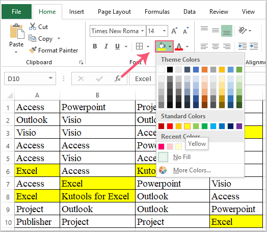
1. Kullanmak istediğiniz veri aralığını seçin ve ardından Giriş > Bul ve Seç > Bul'a tıklayın, ekran görüntüsüne bakın:

2. Bul ve Değiştir iletişim kutusunda, Bul sekmesi altında, Bulunacak metin kutusuna bulmak istediğiniz değeri girin, ekran görüntüsüne bakın:

3. Ve ardından, Tümünü Bul düğmesine tıklayın, bulunan sonuçlar kutusunda herhangi bir öğeye tıklayın ve ardından tüm bulunan öğeleri seçmek için Ctrl + A tuşlarına basın, ekran görüntüsüne bakın:

4. Son olarak, bu iletişim kutusunu kapatmak için Kapat düğmesine tıklayın. Şimdi, bu seçili değerlere bir arka plan veya yazı tipi rengi uygulayabilirsiniz, ekran görüntüsüne bakın:
| Seçili hücreler için arka plan rengini uygulama: | Seçili hücreler için yazı tipi rengini uygulama: |
 |  |
Yöntem 3: Kutools for Excel ile hücre değerine göre arka plan veya yazı tipi rengini statik olarak değiştirme
Kutools for Excel'in Süper Bul özelliği, değerleri, metin dizelerini, tarihleri, formülleri, biçimlendirilmiş hücreleri vb. bulmak için birçok koşulu destekler. Eşleşen hücreleri bulup seçtikten sonra, arka plan veya yazı tipi rengini istediğiniz gibi değiştirebilirsiniz.
1. Bulmak istediğiniz veri aralığını seçin ve ardından Kutools > Süper Bul'a tıklayın, ekran görüntüsüne bakın:

2. Süper Bul panelinde, lütfen aşağıdaki işlemleri yapın:
- (1.) İlk olarak, Değerler seçenek simgesine tıklayın;
- (2.) İçinde açılır menüsünden bulma kapsamını seçin, bu durumda Ben Seçim'i seçeceğim;
- (3.) Tür açılır listesinden kullanmak istediğiniz kriteri seçin;
- (4.) Ardından, tüm ilgili sonuçları liste kutusuna listelemek için Bul düğmesine tıklayın;
- (5.) Son olarak, hücreleri seçmek için Seç düğmesine tıklayın.

3. Ve ardından, kriterlere uygun tüm hücreler bir defada seçildi, ekran görüntüsüne bakın:

4. Ve şimdi, seçili hücreler için arka plan rengini veya yazı tipi rengini ihtiyaçlarınıza göre değiştirebilirsiniz.
İpuçları: Süper Bul işlevi ile aşağıdaki işlemleri de hızlı ve kolay bir şekilde gerçekleştirebilirsiniz:
Daha fazla bilgi edin... İndir ve 60 günlük ücretsiz deneme sürümü
En İyi Ofis Verimlilik Araçları
Kutools for Excel ile Excel becerilerinizi güçlendirin ve benzersiz bir verimlilik deneyimi yaşayın. Kutools for Excel, üretkenliği artırmak ve zamandan tasarruf etmek için300'den fazla Gelişmiş Özellik sunuyor. İhtiyacınız olan özelliği almak için buraya tıklayın...
Office Tab, Ofis uygulamalarına sekmeli arayüz kazandırır ve işinizi çok daha kolaylaştırır.
- Word, Excel, PowerPoint'te sekmeli düzenleme ve okuma işlevini etkinleştirin.
- Yeni pencereler yerine aynı pencerede yeni sekmelerde birden fazla belge açıp oluşturun.
- Verimliliğinizi %50 artırır ve her gün yüzlerce mouse tıklaması azaltır!
Tüm Kutools eklentileri. Tek kurulum
Kutools for Office paketi, Excel, Word, Outlook & PowerPoint için eklentileri ve Office Tab Pro'yu bir araya getirir; Office uygulamalarında çalışan ekipler için ideal bir çözümdür.
- Hepsi bir arada paket — Excel, Word, Outlook & PowerPoint eklentileri + Office Tab Pro
- Tek kurulum, tek lisans — dakikalar içinde kurulun (MSI hazır)
- Birlikte daha verimli — Ofis uygulamalarında hızlı üretkenlik
- 30 günlük tam özellikli deneme — kayıt yok, kredi kartı yok
- En iyi değer — tek tek eklenti almak yerine tasarruf edin