Ana içeriğe atla

Excel'de her ayın ilk veya son cuma günü nasıl bulunur?

Yazarı: Siluvia Son Değiştirilme Tarihi: 2020-07-22

Normalde Cuma, bir ayın son iş günüdür. Excel'de belirli bir tarihe göre ilk veya son Cuma gününü nasıl bulabilirsiniz? Bu yazıda, her ayın ilk veya son Cuma gününü bulmak için iki formülü nasıl kullanacağınız konusunda size rehberlik edeceğiz.

Bir ayın ilk Cuma gününü bulun
Bir ayın son Cuma gününü bulun


Bir ayın ilk Cuma gününü bulun

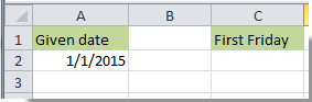
Örneğin, aşağıda gösterilen ekran görüntüsü gibi A1 hücresinde 1/2015/2 belirli bir tarih bulunur. Verilen tarihe göre ayın ilk Cuma gününü bulmak istiyorsanız, lütfen aşağıdaki işlemleri yapın.

1. Sonucu görüntülemek için bir hücre seçin. Burada C2 hücresini seçiyoruz.

2. Aşağıdaki formülü kopyalayıp içine yapıştırın ve ardından Keşfet tuşuna basın.

=CEILING(EOMONTH(A2,-1)-5,7)+6

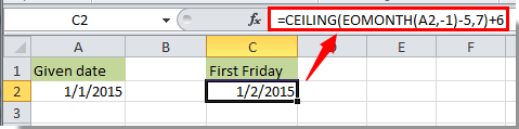
Ardından tarih C2 hücresinde görüntülenir; bu, Ocak 2015'in ilk Cuma gününün 1/2/2015 tarihi olduğu anlamına gelir.

notlar:

1. Diğer ayların ilk Cuma gününü bulmak istiyorsanız, lütfen o ayın belirtilen tarihini A2 hücresine girin ve sonra formülü kullanın.

2. Formülde A2, verilen tarihin bulunduğu referans hücredir. İhtiyaçlarınızı karşılayacak şekilde değiştirebilirsiniz.

Bir ayın son Cuma gününü bulun

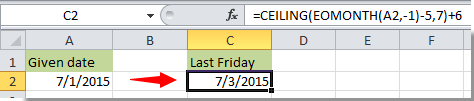
Verilen tarih 1/1/2015, bu ayın son Cuma gününü Excel'de bulmak için A2 hücresinde bulunur, lütfen aşağıdaki işlemleri gerçekleştirin.

1. Bir hücre seçin, aşağıdaki formülü içine kopyalayın ve ardından Keşfet sonucu almak için anahtar.

=DATE(YEAR(A2),MONTH(A2)+1,0)+MOD(-WEEKDAY(DATE(YEAR(A2),MONTH(A2)+1,0),2)-2,-7)

Ardından, 2015 Ocak ayının son Cuma günü B2 hücresini görüntülüyor.

not: Formüldeki A2'yi, verilen tarihin referans hücresiyle değiştirebilirsiniz.


İlgili yazılar:

En İyi Ofis Üretkenlik Araçları

🤖 Kutools AI Yardımcısı: Aşağıdakilere dayalı olarak veri analizinde devrim yaratın: Akıllı Yürütme   |  Kodunu oluşturun  |  Özel Formüller Oluşturun  |  Verileri Analiz Edin ve Grafikler Oluşturun  |  Kutools İşlevlerini Çağır...
Popüler Özellikler: Yinelenenleri Bul, Vurgula veya Tanımla   |  Boş Satırları Sil   |  Veri Kaybı Olmadan Sütunları veya Hücreleri Birleştirin   |   Formülsüz Tur ...
Süper Arama: Çoklu Ölçütlü VLookup    Çoklu Değer VLookup  |   Birden Çok Sayfada VLookup   |   Bulanık Arama ....
Gelişmiş Açılır Liste: Hızla Açılır Liste Oluşturun   |  Bağımlı Açılır Liste   |  Çoklu Seçim Açılır Liste ....
Sütun Yöneticisi: Belirli Sayıda Sütun Ekleme  |  Sütunları Taşı  |  Gizli Sütunların Görünürlük Durumunu Değiştir  |  Aralıkları ve Sütunları Karşılaştırın ...
Öne Çıkan Özellikler: Izgara Odağı   |  Tasarım görünümü   |   Büyük Formül Çubuğu    Çalışma Kitabı ve Sayfa Yöneticisi   |  Kaynak Kütüphanesi (Otomatik metin)   |  Tarih Seçici   |  Çalışma Sayfalarını Birleştirin   |  Hücreleri Şifrele/Şifresini Çöz    E-postaları Listeye Göre Gönder   |  Süper Filtre   |   Özel Filtre (kalın/italik/üstü çizili filtre...) ...
En İyi 15 Araç Seti12 Metin Tools (Metin ekle, Karakterleri Kaldır, ...)   |   50+ Grafik Türleri (Gantt şeması, ...)   |   40+ Pratik Formüller (Yaşı doğum gününe göre hesapla, ...)   |   19 sokma Tools (QR Kodunu Girin, Yoldan Resim Ekle, ...)   |   12 Dönüştürme Tools (Sayılardan Kelimelere, Para Birimi Dönüştürme, ...)   |   7 Birleştir ve Böl Tools (Gelişmiş Kombine Satırları, Bölünmüş hücreler, ...)   |   ... ve dahası

Kutools for Excel ile Excel Becerilerinizi Güçlendirin ve Daha Önce Hiç Olmadığı Gibi Verimliliği Deneyimleyin. Kutools for Excel, Üretkenliği Artırmak ve Zamandan Tasarruf Etmek için 300'den Fazla Gelişmiş Özellik Sunar.  En Çok İhtiyacınız Olan Özelliği Almak İçin Buraya Tıklayın...

Açıklama


Office Tab, Office'e Sekmeli Arayüz Getirir ve İşinizi Çok Daha Kolay Hale Getirir

  • Word, Excel, PowerPoint'te sekmeli düzenlemeyi ve okumayı etkinleştirin, Publisher, Access, Visio ve Project.
  • Yeni pencereler yerine aynı pencerenin yeni sekmelerinde birden çok belge açın ve oluşturun.
  • Üretkenliğinizi% 50 artırır ve her gün sizin için yüzlerce fare tıklamasını azaltır!
Comments (12)
Rated 5 out of 5 · 1 ratings
This comment was minimized by the moderator on the site
Even shorter 😅
=lambda(Date;WeekDay;EOMONTH(Date;0)-WEEKDAY(EOMONTH(Date;0);WeekDay+10)+1
Where "WeekDay" parameter is 1=Monday, 7=Sunday
This comment was minimized by the moderator on the site
=lambda(Date;WeekDay;EOMONTH(Date;0)-WEEKDAY(EOMONTH(Date;0);WeekDay+10)+1)

I forgot a bracket at the end
This comment was minimized by the moderator on the site
Vậy công thức tính thứ sáu tuần thứ 2 của tháng như thế nào vậy ban?
This comment was minimized by the moderator on the site
Hi Tâm Cao Điền,
Suppose you want to calculate the second friday of the month based on the given date in A1, you can try the following formula:
=A18-DAY(A18)+CHOOSE(WEEKDAY(A18-DAY(A18),2),11,10,9,8,14,13,12)
This comment was minimized by the moderator on the site
porque cuando lo pruebo tal cual me sale error ?
o sea estoy copiando y pegando y no funciona

alguien sabe?
This comment was minimized by the moderator on the site
Hi andre,
Can you tell me which formula you used in the post? And what error your are experiencing?
This comment was minimized by the moderator on the site
Why not make the "last Friday" formula: =CEILING(EOMONTH(A2,0)-5,7)-1? That works for all dates I have tried....
This comment was minimized by the moderator on the site
Hi Eric,
I hop you are still on this forum and receive my reply.
Thanks so much for an EASY formula. I've never encountered =CEILING.
Rated 5 out of 5
This comment was minimized by the moderator on the site
Hi Eric,
Thanks for sharing it.
This comment was minimized by the moderator on the site
Hello and thank you for this formula. I am not an Excel guru and acnnot easily work out how to change this formula for the last Friday to be the Last Monday, or any other day. Can you please explain how to interpret this.
This comment was minimized by the moderator on the site
Matt,

The way the formula works is: First we find the last day of the month with the EOMONTH() function. For the last day of the current month, we use "0" as the month offset. For the previous month, it would be -1. (Either "=EOMONTH(A2,0)" or "=EOMONTH(A2,-1)".)

Then, in the "=CEILING()" function, we subtract the number of days required to bring us back to Sunday from the day for which we are searching. (For Tuesday, it would be -2, so we make the formula so far: "=CEILING(EOMONTH(A2,0)-2...."

We use the "significance" value of "7" because weeks are seven days long (of course).This finds the date of either the previous Saturday, or the following Saturday (Excel dates started with 1/1/1900, which was a Sunday. So if you enter a "1" in cell A2 with the Long Date format, the cell would read: "Sunday, January 1, 1900".). For that reason, the =CEILING() function, using "7" as the "significance" argument returns Saturday, which is always a multiple of 7 in Excel. Now the formula is "=CEILING(EOMONTH(A2,0)-2,7...".

Now we need to return the date to a Tuesday, so we either subtract 4 for the last Tuesday of the month, or add 3 for the first Tuesday of the next month. So the final formula is, respectively, either "=CEILING(EOMONTH(A2,0)-2,7)-4" or "=CEILING(EOMONTH(A2,0)-2,7)+3".

We can work through the math by assuming the last day of the month is either a Monday (assume its value is 9 - for ease of illustration, so the values do not go negative) or a Wednesday (assume value 11). "EOMONTH()" will return either of those days (9 or 11). Subtracting 2 results in the previous Saturday (value 7) or Monday (value 9), respectively. The CEILING() function then returns, respectively, the previous Saturday (value 7, because the ceiling of 7 with significance 7 is 7) or the current Saturday (value 14, because the ceiling of 9, significance 7, is 14). Subtracting 4 results in the previous Tuesday (value 3) or the current week's Tuesday (value 10), respectively. For the first Tuesday of the following month, adding 3 to the Saturday value (7 or 14) returns either Tuesday value 10, or Tuesday value 17, respectively.


Hopefully that helps you understand so that you can modify the formula as necessary. You can even change it to find the second Tuesday, or second to last Tuesday, by adding or subtracting an additional 7, respectively.
This comment was minimized by the moderator on the site
Hi Matt,
You just need to change the last number -7 to -1 to solove the problem.
=DATE(YEAR(A2),MONTH(A2)+1,0)+MOD(-WEEKDAY(DATE(YEAR(A2),MONTH(A2)+1,0),2)-2,-1)
There are no comments posted here yet
Please leave your comments in English
Posting as Guest
×
Rate this post:
0   Characters
Suggested Locations